DIFFERENCE Function
Differences a seasonal or nonseasonal time series.
Usage
result = DIFFRENCE(z, periods)
Input Parameters
z—One-dimensional array containing the time series.
periods—One-dimensional array containing the periods at which z is to be differenced.
Returned Value
result—One-dimensional array of length N_ELEMENTS (z) containing the differenced series.
Input Keywords
Double—If present and nonzero, double precision is used.
Orders—One-dimensional array of length N_ELEMENTS(periods) containing the order of each difference given in periods. The elements of Orders must be greater than or equal to 0. Default: all the elements equal 1
Exclude_First, First_To_Nan—If Exclude_First is present and nonzero, the first Num_Lost observations are excluded from the solution due to differencing. The differenced series is of length N_ELEMENTS(periods) – Num_Lost. If First_To_Nan is specified, the first Num_Lost observations are set to NaN (Not a Number). This is the default if neither Exclude_First nor First_To_Nan is specified. Default: First_To_Nan
Output Keywords
Num_Lost—Named variable into which the number of observations “lost” because of differencing the time series z is stored.
Discussion
Function DIFFERENCE performs m = N_ELEMENTS(periods) successive backward differences of period si = periods(i – 1) and di = Orders(i – 1) for i = 1, ..., m on the n = N_ELEMENTS(x) observations {Zt} for t = 1, 2, ..., n. Consider the backward shift operator B given by:
BkZt = Zt – k
for all k. Then, the backward difference operator with period s is defined by the following:

Note that BsZt and ΔsZt are defined only for t = (s + 1), ..., n. Repeated differencing with period s is simply:

where d ≥ 0 is the order of differencing. Note that Δds Zt is defined only for
t = (sd + 1), ..., n.
t = (sd + 1), ..., n.
The general difference formula used in DIFFERENCE is given by:

where nL represents the number of observations “lost” because of differencing and NaN represents the missing value code. See MACHINE to retrieve missing values. Note that:

A homogeneous, stationary time series can be arrived at by appropriately differencing a homogeneous, nonstationary time series (Box and Jenkins 1976, p. 85). Preliminary application of an appropriate transformation followed by differencing of a series enables model identification and parameter estimation in the class of homogeneous stationary ARMA.
Example 1
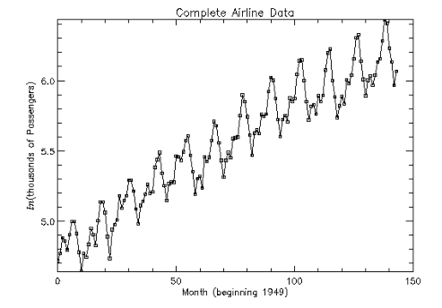
Consider the Airline Data (Box and Jenkins 1976, p. 531) consisting of the monthly total number of international airline passengers from January 1949 through December 1960. The entire data, after taking a natural logarithm, are shown in Figure 9-3: Complete Airline Data Plot. The plot shows a linear trend and a seasonal pattern with a period of 12 months. This suggests that the data needs a nonseasonal difference operator, Δ1, and a seasonal difference operator, Δ12, to make the series stationary. Function DIFFERENCE is used to compute:
Wt = Δ1Δ12Zt = (Zt – Zt – 12) – (Zt – 1 – Zt – 13)
for t = 14, 15, ..., 24.
; Get the data set.
ztemp = ALOG(STATDATA(4))
; Plot the complete data set.
PLOT, INDGEN(144), ztemp, Psym = -6, Symsize = .5, $
YStyle = 1, Title = 'Complete Airline Data', $
XTitle = 'Month (beginning 1949)', $
YTitle = '!8ln!3(thousands of Passengers)'
z = ztemp(0:23)
periods = [1, 12]
; Call DIFFERENCE.
difference = DIFFERENCE(z, periods)
; Create a matrix of the data to make the output easier.
matrix = [[INDGEN(24)], [z], [difference]]
; Output the results.
PM, matrix, Format = '(i4, x, 2f7.1)', $
Title = ' I z(i) difference(i)'
This results in the following output:
I z(i) difference(i)
0 112.0 NaN
1 118.0 NaN
2 132.0 NaN
3 129.0 NaN
4 121.0 NaN
5 135.0 NaN
6 148.0 NaN
7 148.0 NaN
8 136.0 NaN
9 119.0 NaN
10 104.0 NaN
11 118.0 NaN
12 115.0 NaN
13 126.0 5.0
14 141.0 1.0
15 135.0 -3.0
16 125.0 -2.0
17 149.0 10.0
18 170.0 8.0
19 170.0 0.0
20 158.0 0.0
21 133.0 -8.0
22 114.0 -4.0
23 140.0 12.0
 |
Example 2
The data for this example is the same as that for the initial example. The first Num_Lost observations are excluded from W due to differencing, and Num_Lost also is output.
ztemp = STATDATA(4)
z = ztemp(0:23)
periods = [1, 12]
; Use Num_Lost to compute the number of rows in the result
; that have valid values.
diff = DIFFERENCE(z, periods, $
/Exclude_First, Num_Lost = num_lost)
num_valid = N_ELEMENTS(z) - num_lost
; Put the data in one matrix to make printing easier.
matrix = [[INDGEN(num_valid)], [z(0:num_valid-1)], $
[DIFF(0:num_valid-1)]]
PM, matrix, Format = '(i4, x, 2f7.1)', $
Title = ' i z(i) DIFFERENCE(i)'
This results in the following output:
   i    z(i)   DIFFERENCE(i)
0   112.0    5.0
1   118.0    1.0
2   132.0   -3.0
3   129.0   -2.0
4   121.0   10.0
5   135.0    8.0
6   148.0    0.0
7   148.0    0.0
8   136.0   -8.0
9   119.0   -4.0
10   104.0   12.0
Fatal Errors
STAT_PERIODS_LT_ZERO—Parameter periods (#) = #. All elements of Periods must be greater than zero.
STAT_ORDER_NEGATIVE—Parameter order (#) = #. All elements of order must be nonnegative.
STAT_Z_CONTAINS_NAN—Parameter z (#) = NaN; z cannot contain missing values. Other elements of z may be equal to NaN.


