Importing data sources
Describes options available and how to importing certain types of data files.

Explains how to import a data source.
Explains the purpose of the Select Data Sources pane.
Explains how to import an ESRI/Shape file and describes the available options.
Explains how to import a nongeoreferenced image file and describes the available options.
Explains how to import a TIGER/Line® file and describes the available options.
Explains how to import a DXF file and describes the available options.
Explains how to import a Web Map Server image and describes the available options.
Explains how to import layers from a DB2® spatial database and describes the available options.
Explains how to import layers from an Informix® spatial database and describes the available options.
Explains how to import layers from an Oracle® spatial database and describes the available options.
Explains how to import an SVG file and describes the available options.
Explains how to import files of any type using the menus.
Shows you how to use the drag-and-drop mechanism to import a generic file.
Importing a simple data source
The Select Data Sources pane displayed depends on the type of data source you want to import. In most cases this is a simple pane.
To import a simple data source.
1. Choose File>Add Map Data to display the Select Data Sources pane.
2. Browse to the data source you want to open, select it, and click Open.
The Select Data Sources pane
In some cases the Select Data Sources pane is more complex and displays specific options depending on the type data source you choose.
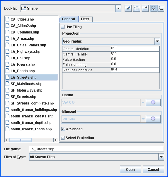
Importing an ESRI/Shape file
If the data source is an ESRI/Shape ( .shp ) file, there are additional options that you can use.
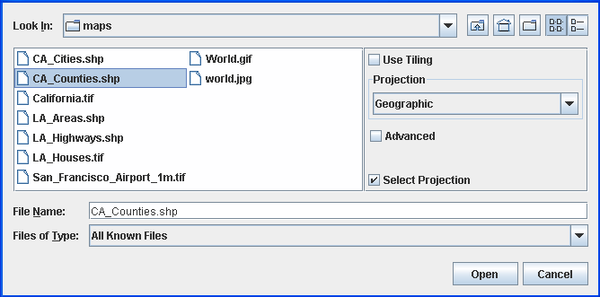
The following figure shows both the Advanced and Select Projection options selected.
Select data sources pane for ESRI/Shape file
1. Choose File>Add Map Data to display the Select Data Sources pane.
2. Select Use Tiling, if you want to have an additional index file ( .idx ) managing the shape file using a load on demand algorithm. If the index file does not exist, the Create index file pane asks you if you want to create a new one.
3. To create a new index file, click Yes to display the Tiling parameters pane and enter the parameters you want.
The following figure shows the Tiling parameters pane.
4. 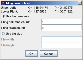
Tiling parameters pane
6. If your shape file has an associated dbf (database) file and thus contains metadata, you can use this to filter so that you load only a subset of the file content. To do this, select the Filter tab, select the Activate Filter check box and define your filter by selecting items from the drop-down lists.
The following figure shows the definition of a filter which will only load San Francisco streets which have ZIP codes greater than ““92000””.
7. 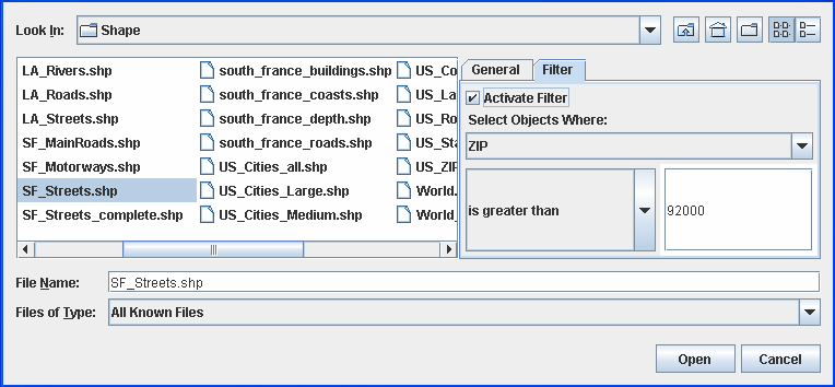
Filter definition to load only a subset of the shape file content
8. Click Open.
Importing nongeoreferenced image files
Explains how to import a nongeoreferenced image file and describes the available options.
Explains how to import a nongeoreferenced image file options.
Describes calibration and image bound options.
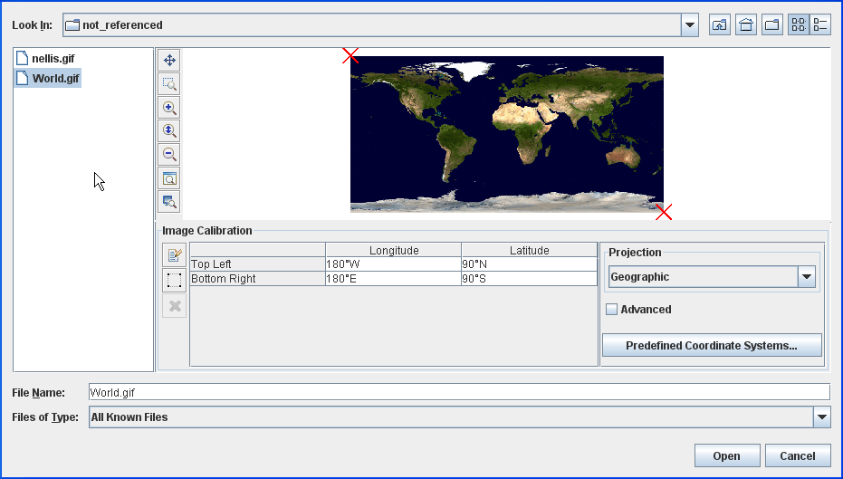
Importing a nongeoreferenced image file
If the data source is a nongeoreferenced image file ( .gif, .tif, .jpg, .jpeg ), there are specific options that you can set.
The following figure shows the options available when importing a nongeoreferenced image file.
Select Data Sources pane for a Nongeoreferenced Image file
1. Choose File>Add Map Data to display the Select Data Sources pane.
2. In the top part of the pane click the gray rectangle to preview the image and use the toolbar to pan, zoom in/out, and fit the image to the view.
3. By default the Image Calibration pane is displayed in bounds mode. In bounds mode you can set the latitude and longitude of the image manually. Click the row and enter the coordinates. You can also click the
4. 
5. button to interactively select the boundaries.
6. To switch to control point mode, click the
7. 
8. button. This adds two columns: Pixel Column and Pixel Line. In this mode you can set the position of the image manually using the pixel properties or the latitude\longitude properties. In addition, you can drag the red crosses to the point you want; this automatically sets the property values in the Image Calibration pane. The red cross associated with a selected row is contained in a rectangle.
9. Click the
10. 
11. button to add another row and another red cross in the Image pane.
12. Click the
13. 14. button again to return to bounds mode.
15. To remove a row from the Image Calibration pane, select the row and click the
16. 
17. button.
18. Since this is a nongeoreferenced data source, you must state the coordinate system in which the data source is defined in the Projection pane. The coordinate system in which you finally project the data source can be a different system and should be defined in the Coordinate System pane, see
Setting coordinate systems.
19. Click Open.
Options when importing a nongeoreferenced image file
Setting the number of calibration points
Calibration in the Image Calibration pane uses an
IlvFittedTransform class. This class requires a certain number of points to be entered for more complex transformations (that is, a higher degree of interpolation).
You must enter:
For a degree 1 polynomial (linear transformation): 3 calibration points.
For a degree 2 polynomial transformation: 6 calibration points.
For a degree 3 polynomial transformation: 10 calibration points.
For a degree 4 polynomial transformation: 15 calibration points.
Polynomial interpolations are more precise in the area inside the calibration points. If you use this feature, try providing calibration points that cover as large an area as possible.
The first part of the following figure shows an initial map of Alaska. Calibration points have been placed around the right side of this image. The second part of the following figure shows the interpolated image, however, the left side is quite skewed.
Setting calibration points
Predefining the Image Bounds Using World Files
World files provide information for image calibration. A World file has the same filename as the main image file. For example, a file called USA.jgw could accompany an image named USA.jpg, and contain the coordinates of the image in seconds of arc.
An example of a World file content is as follows:
1.50000000000000 (X pixel size)
0.00000000000000 (translation)
0.00000000000000 (rotation)
-1.50000000000000 (Y pixel size)
1934001.50000000000000 (X coordinate of the upper left pixel)
1187698.50000000000000 (Y coordinate of the upper left pixel)
The Map Builder ignores the translation and rotation parameters.
When loading images in GIF, JPG, PNG, or TIF format, the Map Builder scans the directory to see if a World file exists, and if so, predefines the image bounds accordingly in the importation dialog box.
For GIF, JPG, PNG, and TIF formats, the world file extensions checked are in the form .tifw or .tfw, .gifw or .gfw, .jpgw or .jgw, and .pngw or .pgw respectively.
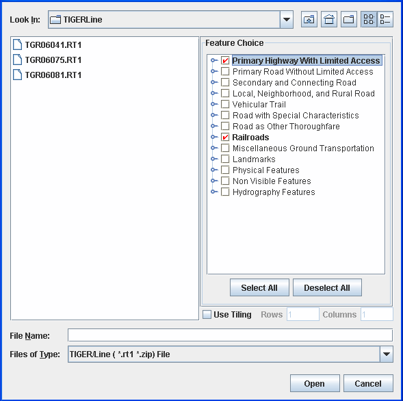
Importing a TIGER/Line file
If the data source is a TIGER/Line® ( *.rt1 ) file, there are specific parameters that you can set.
The following figure shows the options available when importing a TIGER/Line file.
Select Data Sources pane for a TIGER/Line file
1. Choose File>Add Map Data to display the Select Data Sources pane.
2. In the Feature Choice pane, click each of the features you want to display in the TIGER/Line data source. Note that you can expand a feature and select one or more of its subfeatures.
3. Click Select All to select all the features in the pane or Deselect All to deselect all of them.
4. Select Use Tiling, if you want to use this option, and set the number of rows and columns.
5. Click Open.
Importing a DXF file
If the data source is a DXF file, there are additional options that you can set.
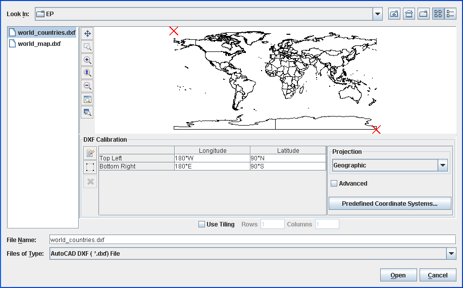
The following figure shows the options available when importing a DXF file.
Select Data Sources pane for a DXF file
1. Choose File>Add Map Data to display the Select Data Sources pane.
2. In the top part of the pane click the gray rectangle to preview the image and use the toolbar to pan, zoom in/out, and fit the image to the view.
3. By default the DXF Calibration pane is displayed in "bounds mode". In bounds mode you can set the latitude and longitude of the image manually. Click the row and enter the coordinates. You can also click the
4. 5. button to interactively select the boundaries.
6. To switch to "control point" mode, click the
7. 8. button. This adds two columns: Pixel Column and Pixel Line. In this mode you can set the position of the image manually using the pixel properties or the latitude\longitude properties. In addition, you can drag the red crosses to the point you want; this automatically sets the property values in the DXF Calibration pane. The red cross associated with a selected row is contained in a rectangle.
9. Click the
10. 11. button to add another row and another red cross in the Image pane.
12. Click the
13. 14. button again to return to bounds mode.
15. To remove a row from the Image Calibration pane, select the row and click the
16. 17. button.
18. Select Use Tiling, if you want to use this option, and set the number of rows and columns.
19. Since this is a nongeoreferenced data source, you must state the coordinate system in which the data source is defined in the Projection pane. The coordinate system in which you finally project the data source can be a different system and should be defined in the Coordinate System pane, see
Setting coordinate systems.
20. Click Open.
Importing a Web Map Server Image
If the data source file is a Web Map Server (WMS) image, there are a number of other parameters that you can set.
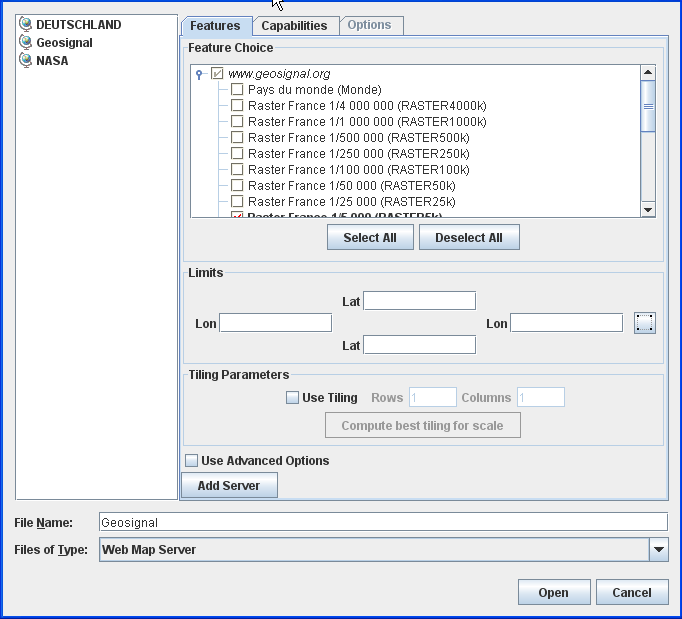
The following figure shows the options available when importing a WMS image.
Select Data Sources pane for a WMS image
In the previous figure the red cross on certain servers indicates that these servers were not available at the time the Map Builder was started.
1. Choose File>Add Map Data and select Web Map Server as the file type, to display the Select Data Sources pane for WMS images.
2. If you need to specify a server that does not appear on the list, click the Add Server button. Enter a name for this server, and the get capabilities URL associated with this server (this information is usually provided by the WMS server).
For instance,
http://wms.jpl.nasa.gov/wms.cgi?request=GetCapabilities
or
http://wms.jpl.nasa.gov/wms.cgi
Click OK to return to server list, where you can select the newly added server.
3. Select a map in the left pane to display the corresponding features in the Features tab, and then select the features you want to display in the Feature Choice pane.
4. Use the Select All button to select all the features or the Deselect All button if you want to remake your selection.
5. Click the Capabilities tab to display the Capabilities pane. The Capabilities pane shows the response from the server to the capabilities request. This pane is for information only and displays the layers that are available in the WMS data.
The following figure shows the Capabilities pane.
6. 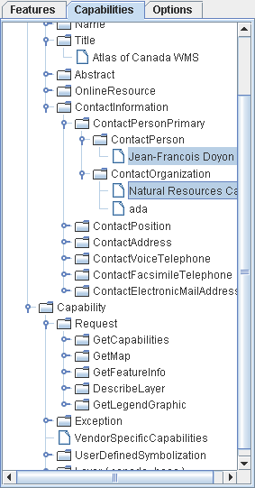
Capabilities pane
7. Select Use Advanced Options, to activate the Options tab and then click the tab to display the Request Options pane. The Request Options pane contains a number of options that you can set.
The following figure shows the Options tab.
8. 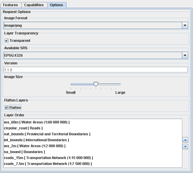
Options pane
9. In the Limits pane, set the limits manually for the Lat/Lon properties or click the
10. 11. button and then draw a rectangle in the Map View to set the limits.
12. To use load-on-demand, select the Use Tiling check box and specify the number and lines and columns of tiles you want to divide the limits region (specified above) into. Given that WMS servers usually limit the image size of a request, this helps improve the overall region resolution by using the specified request image size per tile (one image request per tile load instead of a unique image request for the whole area of interest).
13. If you know the scale you want to display the image at, click Compute best tiling for scale. An Enter Scale input window then opens in which you can enter the desired scale with which the tiling parameters will be computed. According to the image size specified in the advanced Options tab, the Map Builder will compute the tile and column counts so that the overall image will have the desired resolution. The scale should be entered either in decimal format or with the 1/xxx notation.
You can click the Get the view scale button to choose the current view scale.
14. 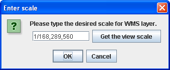
Enter scale pop-up window
15. Set the image format by selecting from the list displayed in the Image Format pane.
16. If you want the layers to be transparent, check the Transparent box in the Layer Transparency pane.
NOTE Transparency is only supported for .gif and .png images. Specifying transparency for other image formats may lead to strange results.
17. Select the Available SRS from the list displayed in the Available SRS pane. The Available SRSs are the available Spatial Reference Systems in which a layer can be displayed. You can only display a layer using one of the SRSs in this list. The list is retrieved from the capabilities request.
18. Set the version number you want in the Version pane. This property allows you to specify the version number as an attribute in the request to the server. Some servers only respond to requests with specific version numbers and reject the request if the version does not match the number they are expecting.
19. In the Image Size pane, set the size of the image by dragging the slider to the required position. This is the size of the image requested on the server and not the size of the image displayed in the Map View. Once read, the image is displayed in the Map View. However, the size of the displayed image does not depend on the size of the requested image since it is georeferenced, but specifying an image size in the request can be useful for tuning the precision versus load time ratio.
20. Check the Flatten box in the Flatten Layers pane to display only one layer for all the selected features. If this option is not checked and you select more than one feature in the Feature pane, a map layer is created for each feature selected.
21. To change the layer order, select a layer in the Layer Order pane and click the
22. 
23. or
24. 
25. button to move the layer up or down one position. Note that to carry out this operation, you must have the Flatten option checked, because the layer order specifies how the features selected in the Features Choice pane are stacked in this single map layer.
26. Click Open.
Importing layers from a DB2 spatial database
If the data source is a DB2®spatial database, there are specific parameters that you can set.
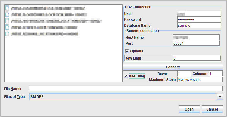
The following figure shows the options available when importing from a DB2 spatial database.
Select Data Sources pane for a DB2 spatial database
To import layers from a DB2 spatial database:
1. Select File>Add Map Data to display the Select Data Sources pane.
2. Choose IBM DB2 in the Files of Type list.
3. Enter the parameters to create a connection to the database. You need a login and a password for the Host machine hosting the database. You will also need the port number and the name of the database.
4. Optionally, if the size of the database is very large, you can specify a Row limit that will limit the number of elements JViews Maps requests from the database at one time. Enter to deactivate that mechanism.
5. Click Connect.
6. If you intend to load data on demand, enable Use Tiling, then specify the column and line count defining the tiling.
7. If you activate tiling, you also have the possibility to specify a maximum scale at which the data will be visible. This will allow you to request the data from the database only when the map sufficiently zoomed. For example, if you enter 1000000, the data will be loaded only if your map is zoomed more than 1/1000,000.
8. Select your table (or tables) and click Open to perform data loading.
NOTE This feature relies on the DB2 JDBC driver that is installed along with
JViews Maps. Please make sure that your DB2 server has a compatible version. See
Requirements for Rogue Wave JViews Maps.
Importing layers from an Informix spatial database
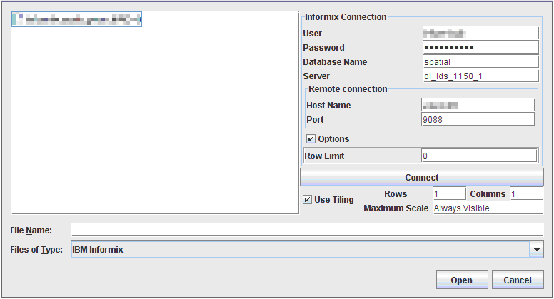
If the data source is an Informix®spatial database, there are specific parameters that you can set. The following figure shows the options available when importing from an Informix spatial database.
Select Data Sources pane for an Informix spatial database
To import layers from an Informix spatial database:
1. Select File>Add Map Data to display the Select Data Sources pane.
2. Choose IBM INFORMIX in the Files of Type list.
3. Enter the parameters to create a connection to the database. You need a login and a password for the Host machine hosting the database. You will also need the port number, the Informix server name and the name of the database.
4. Optionally, if the size of the database is very large, you can specify a Row limit that will limit the number of elements JViews Maps requests from the database at one time. Enter to deactivate that mechanism.
5. Click Connect.
6. If you intend to load data on demand, enable Use Tiling, then specify the column and line count defining the tiling.
7. If you activate tiling, you also have the possibility to specify a maximum scale at which the data will be visible. This will allow you to request the data from the database only when the map sufficiently zoomed. For example, if you enter 1000000, the data will be loaded only if your map is zoomed more than 1/1000,000.
8. Select your table (or tables) and click Open to perform data loading.
Importing layers from an Oracle spatial database
If the data source is an Oracle® spatial database, there are specific parameters that you can set.
The following figure shows the options available when importing from an Oracle Spatial database.
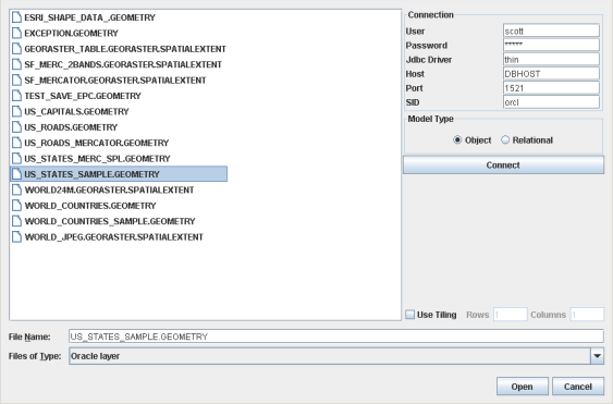
Select Data Sources pane for an Oracle spatial database
To import layers from an Oracle Spatial database:
1. Choose File>Add Map Data to display the Select Data Sources pane.
2. Choose Oracle Layer in the Files of Type list.
3. Enter the parameters to create a connection to the database. You need a login and a password for the Host machine hosting the database. You will also need the port number and the Spatial ID of the database, that is, the "name" of the database.
4. Select the model type of your database. In recent Oracle spatial databases, object model is the standard.
5. Click Connect.
6. If you intend to load data on demand, enable Use Tiling, then specify the column and line count defining the tiling.
7. Click Open to perform data loading.
NOTE before using this functionality, you must install an Oracle driver to be able to import Oracle layers within the Map Builder. For information on how to do this, refer to Importing Oracle Layers within Map Builder in the help file found at
<installdir> /jviews-maps/samples/mapbuilder/index.html.
Importing an SVG file
If the data source is a SVG file, there are additional options that you can set.
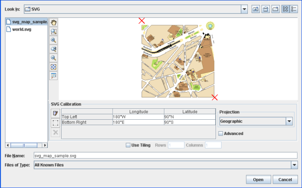
The following figure shows the options available when importing an SVG file.
Select Data Sources pane for an SVG file
1. Choose File>Add Map Data to display the Select Data Sources pane.
2. In the top part of the pane click the gray rectangle to preview the image and use the toolbar to pan, zoom in/out, and fit the image to the view.
3. By default the SVG Calibration pane is displayed in "bounds mode". In bounds mode you can set the latitude and longitude of the image manually. Click the row and enter the coordinates. You can also click the
4. 5. button to interactively select the boundaries.
6. To switch to "control point" mode, click the
7. 8. button. This adds two columns: Pixel Column and Pixel Line. In this mode you can set the position of the image manually using the pixel properties or the latitude\longitude properties. In addition, you can drag the red crosses to the point you want; this automatically sets the property values in the SVG Calibration pane. The red cross associated with a selected row is contained in a rectangle.
9. Click the
10. 11. button to add another row and another red cross in the Image pane.
12. Click the
13. 14. button again to return to bounds mode.
15. To remove a row from the Image Calibration pane, select the row and click the
16. 17. button.
18. Select Use Tiling, if you want to use this option, and set the number of rows and columns.
19. Click Open.
Importing any file type using menus
You can choose to import from files from any data source type by selecting the generic filter “All Known Files” for the file type in the Select Data Sources pane.
The following figure shows the generic filter “All Known Files” for importing any type of file.
The Select Data Sources pane for any known file
To import a file of any known type:
1. Choose File>Add Map Data, the Select Data Sources pane appears.
2. Select one or more file(s).
Depending on the type of file selected, a pane will appear at the right of the Select Data Sources pane.
3. Enter any additional information necessary to open the file.
4. Click Open. After loading, the data source appears in a separate layer of your current map.
Using drag-and-drop
To import a file using drag-and-drop:
Drag a file from your file explorer into the main view window.
If more information is needed to open the file, a specific dialog will appear to allow for this data.
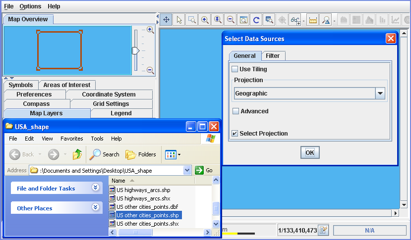
The following figure shows an example of dropping a shape file (.shp) into the main window. You are prompted to specify a projection.
Opening any known file using drag-and-drop
NOTE when you drag and drop IVL files, the Map Builder treats the file as a prepared map. The file is opened and replaces the map currently displayed.
Copyright © 2018, Rogue Wave Software, Inc. All Rights Reserved.