Class
RWLeastSqSVDCalc employs
singular value decomposition (SVD). The method solves the least squares problem by decomposing the regression matrix into the form

, where
P is an

matrix consisting of
p orthonormalized eigenvectors associated with the
p largest eigenvalues of

,
Q is a

orthogonal matrix consisting of the orthonormalized eigenvectors of
, and
Σ = diag(
σ1,
σ2, ... ,
σp) is a

diagonal matrix of singular values of
X. This singular value decomposition of
X is used to solve the equation in
“Calculation Methods for Linear Regression”.
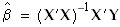
 is equivalent to solving the normal equations
  . Thus the solution for