Multiple Linear Regression
In the late 1880s, Francis Galton was studying the inheritance of physical characteristics. In particular, he wondered if he could predict a boy’s adult height based on the height of his father. Galton hypothesized that the taller the father, the taller the son would be. He plotted the heights of fathers and the heights of their sons for a number of father-son pairs, then tried to fit a straight line through the data. If we denote the son’s height by HS and the father’s height by HF, we can say that in mathematical terms, Galton wanted to determine constants β0 and β1 such that:
HS= β0 + β1HF
This is an example of a simple linear regression problem with a single predictor variable, HF. The parameter β0 is called the intercept parameter. In general, a regression problem may consist of several predictor variables. Thus the multiple linear regression problem may be stated as follows:
Let Y be a random variable that can be expressed in the form:
Y = β0 + β1x1 + ... + βp – 1 + ε
where x1, x2, ... , xp – 1 are known constants, and ε is a fluctuation error. The problem is to estimate the parameters βj. If the xj are varied and the n values Y1, Y2, ..., Yn of Y are observed, then we write:
Yi = β0 + β1xi1 + ... + βp – 1xi, p – 1 + εi (i = 1, 2, ..., n)
where xij is the ith value of xj. Writing these n equations in matrix form we have: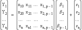
or:
Y = Xβ + ε
where x10 = x20 = ... = xn0 = 1
We call the  matrix X the regression matrix, each Yi a response variable, Y the response vector, and xj the predictor variable.
matrix X the regression matrix, each Yi a response variable, Y the response vector, and xj the predictor variable.


