DCT Function (PV-WAVE Extreme Advantage)

Performs the discrete cosine transform on a 2D image or a 3D array of images.

Usage

result = DCT(array[, direction])

Input Parameters

array—A 2D or 3D array containing an image; or image, row or pixel-interleaved images.

direction—(optional) A scalar value indicating the direction of the transform:

– 1—Forward transform (default)

1—Backward transform

Returned Value

result—A float array of the same size and dimensions as array.

Keywords

Intleave—A scalar string indicating the type of interleaving of 3D input image arrays. Valid strings and the corresponding interleaving methods are:

'pixel'—The input array arrangement is (p, x, y) for p pixel-interleaved images of x-by-y.

'row'—The 3D image array arrangement is (x, p, y) for p row-interleaved images of x-by-y.

'image'—The 3D image array arrangement is (x, y, p) for p image-interleaved images of x-by-y.

Discussion

The discrete cosine transform (DCT) is often used in image compression and coding. A simple compression algorithm truncates a percentage of the coefficients in the DCT result, and then performs an inverse DCT of the truncated array. The quality of the compressed image is related to the percentage of truncated coefficients.

The equation for the DCT is similar to that of the FFT. In two dimensions, the forward transform is defined by the following equation:

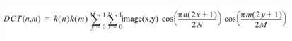
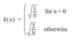
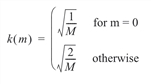
where n and m are defined from 1 to N – 1 and M – 1, respectively and:

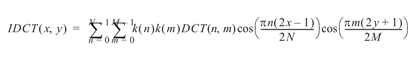
The inverse transform is defined as:

Example

Take the forward DCT of an image.

; Read in an image.

image = IMAGE_READ(!IP_Data + 'face.tif')

; Take the direct cosine transform of the image.

image_dct = DCT(image('pixels'), -1)

; Display the result.

TVSCL, IPALOG(image_dct)

; Take the inverse DCT.

image_idct = DCT(image_dct, 1)

TVSCL, image_idct