CONTOURFILL Procedure

Standard Library procedure that fills both open and closed contours with specified colors or patterns.

Note: CONTOURFS supersedes CONTOURFILL.

Usage

CONTOURFILL, filename, z [, x, y]

Input Parameters

filename—The name of the file containing the contour paths. This file is created using the CONTOUR procedure with the Path_Filename keyword.

z—A 2D array used to generate the contour surface. This array is the same as the one used by CONTOUR.

x—(optional) A vector specifying the x-coordinates used to generate the contours. This vector is the same as the one used by CONTOUR.

y—(optional) A vector specifying the y-coordinates used to generate the contours. This array is the same as the one used by CONTOUR.

Keywords

Color_Index—If present, specifies an array containing the color indices to be used in the plot. Element i of this array contains the color of contour level number i – 1. Element 0 contains the background color. There must be one more color index than there are number of contour levels.

If not present, the contour colors span the range of available colors.

Delete_File—If present, deletes filename after the CONTOURFILL procedure finishes.

Pattern—(UNIX only) A 3D array containing the patterns used to fill the various contour levels. Each pattern is an n-by-m rectangular array of pixels. (See the description of the Pattern graphics keyword in Graphics and Plotting Keywords for an example.)

If NP number of patterns are specified, Pattern will be dimensioned (n, m, NP). The patterns are used to fill the various contour levels. If there are more levels than patterns, the patterns will be cyclically repeated.

XRange and YRange—The desired data range of the x and y-axes, specified as a two-element vector. The first element is the axis minimum, and the second is the maximum. PV‑WAVE will frequently round this range. You must use the XRange and YRange keywords with CONTOURFILL if:

The XRange and YRange keywords are used in the CONTOUR procedure call that is used to generate input for CONTOURFILL.
XRange and YRange are different from the array bounds of the z parameter (the contour surface data), or the minimum and maximum of the x and y parameters, when given.

Defaults: When the z parameter has dim₁ = nx and dim₂ = ny, XRange=[0, nx–1] and YRange=[0, ny–1]. When x and y parameters are given, XRange=[MIN(x), MAX(x)] and YRange=[MIN(y), MAX(y)].

Note: For best results, the XRange and YRange keywords used with CONTOURFILL should match the ones used with CONTOUR.

Discussion

CONTOURFILL can be used with CONTOUR to fill the area between the contour lines with a solid color or a user-defined pattern. The procedure closes the open contours as long as the z (and x and y, if used in the calling sequence) parameter is specified in exactly the same manner as was used with the CONTOUR procedure.

Note:

If you are plotting a large data set, use the EMPTY procedure to be sure that all buffered output is written to the current graphics device.

CONTOURFILL creates a temporary file named filename+1, so you must have write permission in the directory where filename exists.

Example 1

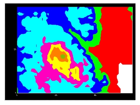
This example creates a contour plot of the Pike’s Peak elevation demo file, with the area in between the contour lines filled with a solid color. The results are shown in Pike’s Peak Contour Plot. The contour plot of Pike’s Peak elevation is filled with solid colors.

; Read in the data file.
OPENR, 1, !Data_dir + 'pikeselev.dat'
pikes = FLTARR(60, 40)
READF, 1, pikes
CLOSE, 1
; Load a color table.
TEK_COLOR
; Contour the data and store the results in file path.dat.
CONTOUR, pikes, Levels=[5,6,7,8,9,10,11,12,13,14,15]*1000,  $
   Path='path.dat', XStyle=1, YStyle=1
; Display contour plot with contours filled with solid colors.
CONTOURFILL, 'path.dat', pikes, $
   Color_Index=WoColorConvert(INDGEN(12))

Pike’s Peak Contour Plot

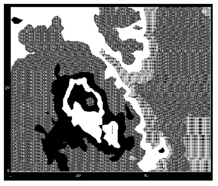
The following commands fill in the area in between the contour lines with a user-defined pattern as shown in Pattern Filled Contour Map of Pike’s Peak’s Elevation. This example only work on UNIX.

; Create the first pattern, a cross pattern.
pat1 = BYTARR(3, 3)
pat1(1, *) = 255
pat1(*, 1) = 255

; Create the second pattern, a diagonal pattern.
pat2 = BYTARR(3, 3)
FOR i=0L, 2 DO pat2(i, i) = 255

; Create the third pattern, a solid fill of color zero.
pat3 = BYTARR(3, 3)

; Create the fourth pattern, a solid fill of color 255.
pat4 = REPLICATE(255b, 3, 3)

; Create the fifth pattern, a backwards diagonal pattern.
pat5 = BYTARR(3, 3)
FOR i=0L, 2 DO pat5(2-i, i) = 255

; Create a 3D array in which to store the patterns.
pat3d = BYTARR(3, 3, 5)

; Store the patterns in the array named pat3d.
pat3d(*, *, 0) = pat1
pat3d(*, *, 1) = pat2
pat3d(*, *, 2) = pat3
pat3d(*, *, 3) = pat4
pat3d(*, *, 4) = pat5

; Display the contour plot with the contours lines filled with
; the pattern.
CONTOURFILL, 'path.dat', pikes, Pattern=pat3d, /Delete_File

Pattern Filled Contour Map of Pike’s Peak’s Elevation

Example 2

Instead of using CONTOURFILL to create color-filled contour plots, a similar result can be achieved by loading a color table with the TEK_COLOR and then using a command of the form:

TV, BYTSCL(array, Top=n)

where n + 1 equals the number of contour levels to be colored.

In other words, the previous example could be displayed using the commands:

TEK_COLOR
pikes=REBIN(pikes, 600, 400)
TV, BYTSCL(pikes, Top = 10)

Some of the advantages of using this technique to create color-filled contour plots, instead of the CONTOURFILL procedure, are:

Easier access to image processing routines that allow you to quickly analyze your data, such as: DEFROI, HISTOGRAM, and PROFILES.
You don’t have to create a temporary file in your directory.