CONTOUR2 Procedure
Draws a contour plot from data stored in an array.
Usage
CONTOUR2, z[, x, y]
Input Parameters
z—A 1D or 2D array containing values of the dependent variable z=z(x, y).
x—A 1D or 2D array containing values of the first independent variable. If z is 1D, then x is a required 1D input variable with the same number of elements as z. If z is 2D, then x is an optional 1D or 2D input.
y—A 1D or 2D array containing values of the second independent variable. If z is 1D, then y is a required 1D input variable with the same number of elements as z. If z is 2D, then y is an optional 1D or 2D input.
Keywords
C_Fillcolors—Specifies an array of color indices used to fill the contour intervals.
Fill—Fills contour intervals with color. This keyword can have the following values:
note | If Fill is specified, labeling is disabled. See Example 2 for information on creating a filled contour plot with labels. |
Frequency—A floating-point value > 0.0 that determines how frequently labels are printed along the contour. If z is an m-by-n array, the default Frequency value is: MIN(m,n)/3.5. If z is a 1D array of length m, the default Frequency value is: SQRT(m)/3.5.
Label_style—An integer specifying the contour label fill style. Possible values are:
The CONTOUR2 keywords let you control many aspects of the contour plot’s appearance. For a description of each keyword, see Chapter 21: Graphics and Plotting Keywords.
Discussion
CONTOUR2 is an implementation of an algorithm developed by Dr. Albrecht Preusser, "Computing area filling contours for surfaces defined by piecewise polynomials", Computer Aided Geometric Design 3 (1986), pp. 267-279.
CONTOUR2 provides functionality that CONTOUR does not. CONTOUR accepts only gridded data: the x and y arrays must define a curvilinear coordinate system. CONTOUR2 places no such restriction on x and y, and thus accepts scattered data as well as gridded data.
For scattered data z, x, and y are 1D arrays of the same length.
For gridded data z is a 2D (m by n) array, while x and y can be 2D, 1D, or undefined. If x and y are 2D then they are of dimensions m by n, and z(i,j) corresponds to the point ( x(i,j), y(i,j) ). If x and y are 1D then they are of lengths m and n respectively, and z(i,j) corresponds to the point ( x(i), y(j) ). If x and y are undefined then they default to x = FINDGEN(m) and y = FINDGEN(n).
Example 1
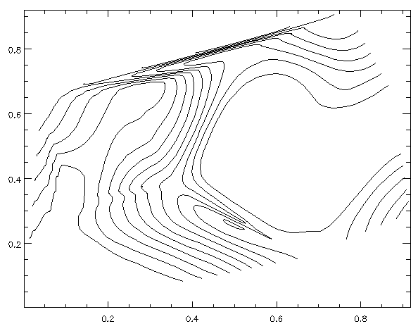
In the example below, randomly scattered data is contoured as shown in Figure 4-4: Contour Plot of Randomly Scattered Data.
seed0 = 0 & seed1 = 2 & seed2 = 5
z = RANDOMU(seed0, 20)
x = RANDOMU(seed1, 20)
y = RANDOMU(seed2, 20)
CONTOUR2, z, x, y, Nlevels=10, /XStyle, /YStyle
 |
Example 2
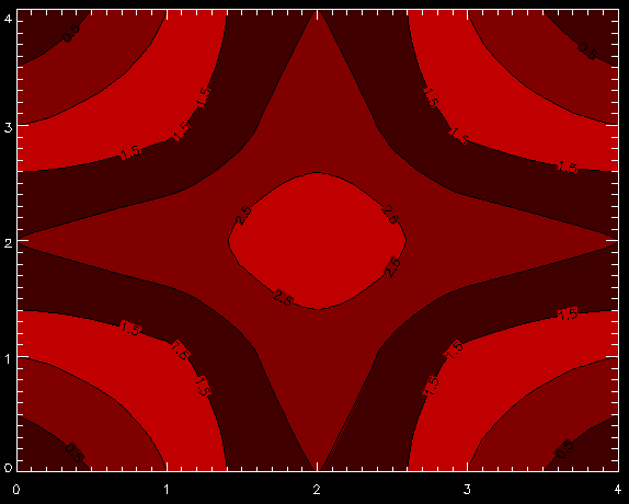
In this example, a filled contour plot with labels is plotted as shown in Figure 4-5: Contour Plot with Labels and Fill Color. Labeling is not active for filled plots, so we’ll generate the filled plot first, then plot the contour lines with labels over the filled plot using the NoErase keyword. We’ll slightly enlarge the size and thickness of the contour labels without affecting the axis text by using the C_Charsize and C_Charthick keywords.
; Define a color table.
TEK_COLOR
z = DIST(5)
colorindex=[20, 21, 22]
; Generate a filled plot with no contour lines.
CONTOUR2, z, /XStyle, /YStyle, NLevels=5, Fill=2, $
C_Fillcolors=colorindex
; Fill contour labels with colors defined in colorindex array.
CONTOUR2, z, /XStyle, /YStyle, NLevels=5, Label_style=3, $
/NoErase, C_Colors=0, C_Fillcolors=colorindex, $
C_Charsize=1, C_Charthick=1
 |
See Also
For more information on contour plots, see the PV‑WAVE User’s Guide.


