GARCH Function
Compute estimates of the parameters of a GARCH(p,q) model.
Usage
result = GARCH(p, q, y, xguess)
Input Parameters
p—Number of autoregressive (AR) parameters.
q—Number of moving average (MA) parameters.
y—One-dimensional array containing the observed time series data.
xguess—One-dimensional array of length p + q + 1 containing the initial values for the parameter array x.
Returned Value
result—One-dimensional array of length p + q + 1 containing the estimated values of sigma squared, followed by the q ARCH parameters, and the p GARCH parameters.
Input Keywords
Double—If present and nonzero, double precision is used.
Max_Sigma—Value of the upperbound on the first element (sigma) of the array of returned estimated coefficients. Default: Max_Sigma = 10.
Output Keywords
Log_Likelihood—Named variable into which the value of Log-likelihood function evaluated at the estimated parameter array x is stored.
Aic—Named variable into which the value of Akaike Information Criterion evaluated at the estimated parameter array x is stored.
Var—Named variable into which an array of size (p + q + 1) by (p + q + 1) containing the variance-covariance matrix is stored.
Discussion
The Generalized Autoregressive Conditional Heteroskedastic (GARCH) model is defined as:

where zt’s are independent and identically distributed standard normal random variables:

The above model is denoted as GARCH(p,q). The p is the autoregressive lag and the q is the moving average lag. When βi = 0, i = 1,2, …, p, the above model reduces to ARCH(q) which was proposed by Engle (1982). The nonnegativity conditions on the parameters implied a nonnegative variance and the condition on the sum of the βi’s and α i’s is required for wide sense stationarity.
In the empirical analysis of observed data, GARCH(1,1) or GARCH(1,2) models have often found to appropriately account for conditional heteroskedasticity (Palm 1996). This finding is similar to linear time series analysis based on ARMA models.
It is important to notice that for the above models positive and negative past values have a symmetric impact on the conditional variance. In practice, many series may have strong asymmetric influence on the conditional variance. To take into account this phenomena, Nelson (1991) put forward Exponential GARCH (EGARCH). Lai (1998) proposed and studied some properties of a general class of models that extended linear relationship of the conditional variance in ARCH and GARCH into nonlinear fashion.
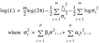
The maximal likelihood method is used in estimating the parameters in GARCH(p,q). The log-likelihood of the model for the observed series {Yt} with length m is:

In the model, if q = 0, the model GARCH is singular such that the estimated Hessian matrix H is singular.
The initial values of the parameter array x entered in array xguess must satisfy certain constraints. The first element of xguess refers to sigma and must be greater than zero and less than Max_Sigma. The remaining p + q initial values must each be greater than or equal to zero but less than one.
To guarantee stationarity in model fitting:

is checked internally. The initial values should be selected from the values between zero and one. The Aic is computed by:
2 * log (L) + 2 * (p+q+1)
where log(L) is the value of the log-likelihood function at the estimated parameters.
In fitting the optimal model, the subroutine MINCONGEN as well as its associated subroutines are modified to find the maximal likelihood estimates of the parameters in the model. Statistical inferences can be performed outside the routine GARCH based on the output of the log-likelihood function (Log_Liklihood), the Akaike Information Criterion (Aic), and the variance-covariance matrix (Var).
Example
The data for this example are generated to follow a GARCH(p,q) process by using a random number generation function SGARCH. The data set is analyzed and estimates of sigma, the AR parameters, and the MA parameters are returned. The values of the Log-likelihood function and the Akaike Information Criterion are returned from the output keywords Log_Likelihood and Aic respectively.
note | To run this example, use the .RUN command and then copy and paste this example into . |
FUNCTION SGARCH, p, q, m, x
z = FLTARR(m + 1000)
y0 = FLTARR(m + 1000)
sigma = FLTARR(m + 1000)
z = RANDOM(m + 1000, /Normal)
l = ((p > q) > 1)
y0(0:l - 1) = z(0:l - 1)*x(0)
; Compute the Initial Value Of Sigma
s3 = 0.0
IF ((p > q) GE 1) THEN s3 = TOTAL(x(1:p + q))
sigma(0:l - 1) = x(0)/(1.0 - s3)
FOR i=l, (m + 1000 - 1) DO BEGIN
s1 = 0.0
s2 = 0.0
IF (q GE 1) THEN BEGIN
FOR j=0L, q - 1 DO s1 = s1 + x(j + 1) * $
(y0(i - j - 1)^2)
END
IF (p GE 1) THEN BEGIN
FOR j=0L, p - 1 DO s2 = s2 + x(q + 1 + j) $
* sigma(i - j - 1)
END
sigma(i) = x(0) + s1 + s2
y0(i) = z(i)*SQRT(sigma(i))
END
; Discard the first 1000 Simulated Observations
RETURN, y0(1000:*)
; End of function
END
RANDOMOPT, Set = 182198625
p = 2
q = 1
m = 1000
x = [1.3, 0.2, 0.3, 0.4]
xguess = [1.0, 0.1, 0.2, 0.3]
y = SGARCH(p, q, m, x)
result = GARCH(p, q, y, xguess, Log_Likelihood = a, Aic = aic)
PRINT, 'Sigma estimate is', result(0)
; PV-WAVE prints: Sigma estimate is 1.75152
PRINT, 'AR(1) estimate is', result(1)
; PV-WAVE prints: AR(1) estimate is 0.249741
PRINT, 'AR(2) estimate is', result(2)
; PV-WAVE prints: AR(2) estimate is 0.325689
PRINT, 'MA(1) estimate is', result(3)
; PV-WAVE prints: MA(1) estimate is 0.313778
PRINT, 'Log-likelihood function value is', a
; PV-WAVE prints: Log-likelihood function value is -2707.08
PRINT, 'Akaike Information Criterion value is', aic
; PV-WAVE prints the following:
; Akaike Information Criterion value is 5422.16


