MVAR_NORMALITY Function
Computes Mardia’s multivariate measures of skewness and kurtosis and tests for multivariate normality.
Usage
result = MVAR_NORMALITY(x)
Input Parameters
x—2D array containing data in which N_ELEMENTS(x(*,0)) is the number of observations (numbers of rows of data) in x and N_ELEMENTS(x(0,*)) is the dimenionality of the multivariate space for which the skewness and kurtosis are to be computed (number of variables in x).
Returned Value
result—One-dimensional array of size 13 containing output statistics as shown in Table 8-1: Output Statistics.
I | result ( I ) |
|---|---|
0 | estimated skewness |
1 | expected skewness assuming a multivariate normal distribution |
2 | asymptotic chi-squared statistic assuming a multivariate normal distribution |
3 | probability of a greater chi-squared |
4 | Mardia and Foster's standard normal score for skewness |
5 | estimated kurtosis |
6 | expected kurtosis assuming a multivariate normal distribution |
7 | asymptotic standard error of the estimated kurtosis |
8 | standard normal score obtained from result(5) through result(7) |
9 | p-value corresponding to result(8) |
10 | Mardia and Foster's standard normal score for kurtosis |
11 | Mardia's SW statistic based upon result(4) and result(10) |
12 | p-value for result(11) |
Input Keywords
Double—If present and nonzero, double precision is used.
Frequencies—One-dimensional array containing the frequencies. Frequencies must be an integer value. Default assumes all Frequencies equal one.
Weights—One-dimensional array containing the weights. Weights must be non-negative. Default assumes all Weights equal one.
Output Keywords
Sum_Freqs—Named variable into which the sum of the frequencies of all observations used in the computations is stored.
Sum_Weights—Named variable into which the sum of the weights times the frequencies for all observations used in the computations is stored.
Nmissing—Named variable into which the number of rows of data in x containing any missing values (NaN) is stored.
Means—Named variable into which a one-dimensional array of length N_ELEMENTS(x(0,*)) containing the sample means is stored.
R_Matrix—Named variable into which an upper triangular array containing the Cholesky RTR factorization of the covariance matrix is stored.
Discussion
MVAR_NORMALITY computes Mardia’s (1970) measures b1,p and b2,p of multivariate skewness and kurtosis, respectfully, for p = N_ELEMENTS(x(0,*)). These measures are then used in computing tests for multivariate normality. Three test statistics, one based upon b1,p alone, one based upon b2,p alone, and an omnibus test statistic formed by combining normal scores obtained from b1,p and b2,p are computed. On the order of np3, operations are re-quired in computing b1,p when the method of Isogai (1983) is used, where n = N_ELEMENTS(x(*,0)). On the order of np2, operations are required in computing b2,p.
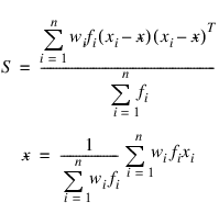
Let:

where:

fi is the frequency of the ith observation, and wi is the weight for this observation. (Weights wi are defined such that xi is distributed according to a multivariate normal, N(μ, Σ/wi) distribution, where Σ is the covariance matrix.) Mardia’s multivariate skewness statistic is defined as:

while Mardia’s kurtosis is given as:

Both measures are invariant under the affine (matrix) transformation AX + D, and reduce to univariate measures when p = N_ELEMENTS(x(0,*)) = 1. Using formulas given in Mardia and Foster (1983), the approximate expected value, asymptotic standard error, and asymptotic p-value for b2,p, and the approximate expected value, an asymptotic chi-squared statistic, and p-value for the b1,p statistic are computed. These statistics are all computed under the null hypothesis of a multivariate normal distribution. In addition, standard normal scores W1(b1,p) and W2(b2,p) (different from but similar to the asymptotic normal and chi-squared statistics above) are computed. These scores are combined into an asymptotic chi-squared statistic with two degrees of freedom:

This chi-squared statistic may be used to test for multivariate normality. A p-value for the chi-squared statistic is also computed.
Example
In the following example, 150 observations from a 5 dimensional standard normal distribution are generated via routine RANDOM. The skewness and kurtosis statistics are then computed for these observations.
m = 150
n = 5
RANDOMOPT, set = 123457
x = FLTARR(n, m)
x(*) = RANDOM(m*n, /Normal)
x = TRANSPOSE(x)
stats = MVAR_NORMALITY(x, Sum_Weights = sw, Sum_Freq = sf, $
Means = means, R_Matrix = r_mat)
PRINT, 'Sum of Frequencies =', sf, Format = '(A25, I4)'
; PV-WAVE prints: Sum of Frequencies = 150
PRINT, 'Sum of the weights =', sw, Format = '(A25, F8.3)'
; PV-WAVE prints: Sum of the weights = 150.000
FOR i=0L, 12 DO PM, i, stats(i), Format = '(I5, F10.2)'
; PV-WAVE prints the following:
; 0 0.73
; 1 1.36
; 2 18.62
; 3 0.99
; 4 -2.37
; 5 32.67
; 6 34.54
; 7 1.27
; 8 -1.48
; 9 0.14
; 10 1.62
; 11 8.24
; 12 0.02


