WgSplineTool Procedure
Graphical User Interface (GUI) that computes a one-dimensional, least-squares spline fit to (possibly noisy) data.
Usage
WgSplineTool[, fit, parent, shell]
Input Parameters
parent—Widget handle of a parent widget. If supplied, it will be used as the parent shell for the tool.
Output Parameters
fit—Structure containing the computed spline. See the introduction of this chapter for a complete description of the spline structure.
shell—Used to pass the shell widget handle for the tool back to the caller.
Input Keywords
XData—One-dimensional array containing the abscissas of the data to be fit. If XData is specified, then YData must also be specified.
YData—One-dimensional array containing ordinates of the data to be fit.
XSize—Width, in pixels, of the draw widget used to display the fit. Keyword XSize must be between 100 and 800. Default: XSize = 600
YSize—Height, in pixels, of the draw widget used to display the fit. Keyword YSize must be between 100 and 800. Default: YSize = 600
Demo_Data—If present and nonzero, sets path to the PV‑WAVE example data directory for importing data. Otherwise, WwFileSelection prompts for input from the same directory from which WgSplineTool was invoked.
Foreground—Specifies the default foreground color name.
Background—Specifies the default background color name.
Font—Specifies the name of the default font used for text.
Position—Specifies the position of the upper-left corner of the main window on the screen.
Title—String specifying shell title. Default is “Constrained Spline Tool.”
Discussion
Procedure WgSplineTool is designed to help compute a least-squares spline fit to (possibly noisy) data. The WgSplineTool procedure computes the fit using function CONLSQ. The default use of WgSplineTool does not require any arguments or keywords and can be used as follows:
WgSplineTool
There are two ways to supply data to WgSplineTool. First, if the data is contained in variables, for example, x and y, invoke WgSplineTool with the following call:
WgSplineTool, XData = x, YData = y
The variables x and y should be one-dimensional arrays of equal length.
The YData keyword can be used without the XData keyword. in this case, it is assumed that the associated x values are monotonically increasing from 0. The call would be as follows:
WgSplineTool, YData = y
The variable y should be a one-dimensional array.
The second method to import data into the application is through an external ASCII file, along with the button labeled Open. The structure of the file is as follows:
For example, the following six lines could be put into a file for use by WgSplineTool:
5
0.0454 3.43245
0.1243 4.45645
0.2454 1.43553
1.2311 1.76543
2.4325 9.53234
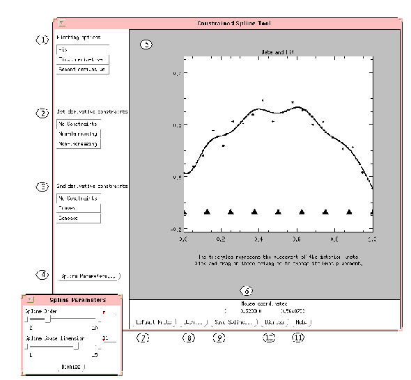
Once the data has been imported to the application, the data is automatically fitted with the default choice of knots. After this is accomplished, you have the ability to add the order of the fit, the spline space dimension, and the placement of the knots. To adjust the placement of the knots, simply use the mouse to “click and drag” the knots on the plot (the knot abscissae are the triangles that appear near the bottom of the plot). WgSplineTool returns the last computed fit in the argument fit.
Use the Save Spline button to save any intermediate fits. After saving the fit, you can restore the spline at a later time into a variable using the following command:
RESTORE, 'filename'
A description of each element of the top-level widget follows. The numbers correspond to the labels in Figure 4-15: Spline Fitting Widget:
 |


