HISTOGRAM Function
Returns the density function of an array.
Usage
result = HISTOGRAM(array)
Input Parameters
array—The array for which the density function will be computed. The size of each dimension of array may be any integer value.
Returned Value
result—A longword vector equal to the density function of the input array.
Keywords
Armax—An array of the maximum values to consider for each image or signal in array. If Armax is a single element array, Armax(0) is used for every image or signal. For a multi-image or multi-signal input array, Armax must contain the same number of elements as there are images or signals in array.
note | When both Armin and Armax are supplied, they must contain the same number of elements. |
Armin—An array of the minimum values to consider for each image or signal in array. If Armin is a single element array, Armin(0) is used for every image or signal. For a multi-image or multi-signal input array, Armin must contain the same number of elements as there are images or signals in the input array.
Binsize—The range of values to consider as having a single value. If no value is specified, the Binsize range defaults to a value of 1.
note | Bins are not right-boundary inclusive. result(i) counts an array value p if: a ≤ p < b where a and b are the lower and upper bin boundaries of the ith bin. See the Inclusive keyword to have the last bin be right-boundary inclusive. |
Inclusive—If set and nonzero, the last bin is right-boundary inclusive. By default, HISTOGRAM counts a datapoint p if a ≤ p < b where a and b are the lower and upper bin boundaries of a given bin.
Intleave—(If used, requires the Armin and Armax keywords.) A scalar string indicating the type of interleaving of 2D input signals containing signal-interleaved signals; and 3D input arrays containing image-interleaved images, or a volume. Valid strings and the corresponding interleaving methods are:
 'signal'
—The 2D input
image array arrangement is (
x,
p) for
p signal-interleaved signals of length
x.
 'image'
—The 3D
image array arrangement is (
x,
y,
p) for
p image-interleaved images of
x-by-
y.
 'volume'
—The input image array is treated as a single entity.
Max—The maximum value to consider. If set but no value is specified, array is searched for its largest value. If the Max keyword is specified, its value is used for every signal or image in the array.
Min—The minimum value to consider. If set but no value is specified, array is searched for its smallest value. If the Min keyword is specified, its value is used for every signal or image in the array.
Omax—Specifies a variable used to hold the maximum value considered in the array. (Equal to max when the Max keyword is given.) If the input array is composed of multiple images or signals, Omax is an array of the maximum values, one for each signal or image. (Equal to max or armax when Max or Armax is given.)
Omin—Specifies a variable to hold the minimum value considered in the array. (Equal to min when Min is given.) If the input array is composed of multiple images or signals, Omin will be an array of the minimum values, one for each signal or image. (Equal to min or armin when Min or Armin is given.)
Discussion
The HISTOGRAM function supports input arrays composed of multiple images (multi-layer band interleaved images) as well as input arrays composed of multiple signals. The Intleave keyword is used to specify whether that the input array is a multi-signal or multi-image array. When the Intleave keyword is used to indicate multiple signals or images in this way, each signal or image in the array is operated on separately and an array of the individual results is returned.
In the simplest case (in which array ranges in value from 0 to some maximum value), the value of the density function at subscript i is equal to the number of array elements with a value of i.
For example, let Fi equal the value of element i, for i in the range {0 ... n–1}. Then Hv (the result of the HISTOGRAM function) is given by:
where:
and P(Fi , v) = 1 when:
and P(Fi , v) = 0 otherwise.
note | There may not always be enough virtual memory available to create density functions of arrays that contain a large number of bins. For information on virtual memory and PV-WAVE, see the PV‑WAVE Programmer’s Guide. |
note | If the range of your data is larger than can be represented by a value of that type, you must promote the type of your data. For example: a = HISTOGRAM([-1, 32767]) The type of this data is a PV-WAVE INT, but the range is larger than an INT can represent. To do this you must promote your data to INT32s or LONGs: a = HISTOGRAM([-1i, 32767]) or a = HISTOGRAM([-1L, 32767]) |
Sample Usage
Histograms are useful in a variety of applications, and can often provide signs as to what type of image processing should be performed. For example, photos sent back via satellite from outer space are usually accompanied by histograms. If the histogram for a photo contains a large spike, and the rest of the histogram is generally flat, this typically indicates that a histogram equalizing operation (such as the HIST_EQUAL function) is needed. Such an operation would spread out the pixels more evenly, thereby improving contrast and bringing out greater detail in the image.
Histograms can also be used to provide clues about images. For example, running a histogram on a series of identical photos taken at different times of the day may show the histogram peak shifting to the right—an indication that the average brightness is higher in that photo, and therefore more likely to be have been taken at a sunnier part of the day.
Similarly, you can use histograms to compare two images of the same scene more fairly. By shifting the histogram of one scene so that it is aligned with that of the other scene, you can equalize the level of brightness in both images.
note | Numerical roundoff errors are inevitable and may cause unexpected results, especially when dealing with base two computation with non-powers of two. For example: h1 = HISTOGRAM(data, min=0, max=1, binsiz=0.1) This statement should return eleven bins but only returns ten. This is due to numerical roundoff errors. These errors are inevitable in base two computations with integers with an odd value. |
Example 1
The data for this example is from Hinkley (1977) and Velleman and Houglin (1981). Data includes measurements (in inches) of precipitation in Minneapolis/St. Paul during the month of March for 30 consecutive years.
; Create sample data.
x = [0.77, 1.74, 0.81, 1.20, 1.95, 1.20, 0.47, 1.43, 3.37, $
2.20, 3.00, 3.09, 1.51, 2.10, 0.52, 1.62, 1.31, 0.32, $
0.59, 0.81, 2.81, 1.87, 1.18, 1.35, 4.75, 2.48, 0.96, $
1.89, 0.90, 2.05]
; Call HISTOGRAM and print the result.
table = HISTOGRAM(x, Binsize = 0.444)
PRINT, ' Bin Number Count' &$
PRINT, ' ---------- -----' &$
FOR i=1L, 10 DO PRINT, i, table(i-1)
; PV-WAVE prints:
; Bin Number Count
; ---------- -----
; 1 4
; 2 8
; 3 5
; 4 5
; 5 3
; 6 1
; 7 3
; 8 0
; 9 0
; 10 1
Example 2
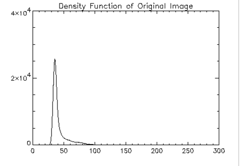
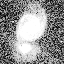
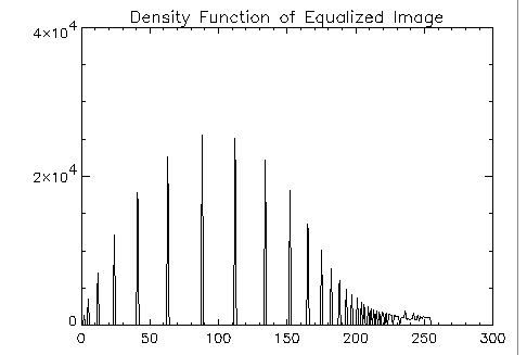
This example exhibits how histogram equalization of an image better distributes pixel values. An image of a galaxy is read and displayed, then the density function of that image is plotted. After the image is histogram equalized, it is displayed, along with a plot of the density function of the equalized image. The results are shown in
Figure 9-2: Original Image Density Function on page 576,
Figure 9-3: Histogram Equalized Galaxy Image on page 576, and
Figure 9-4: Density Function Plot on page 577.
; Open the file containing the galaxy image.
OPENR, unit, !Data_dir + 'whirlpool.img', /Get_Lun
; Create an array large enough to hold the image.
g = BYTARR(512, 512)
; Read the image.
READU, unit, g
; Close the file and free the file unit number.
FREE_LUN, unit
!Order = 1
; Create a window with the same dimensions as the image.
WINDOW, 0, Xsize=512, Ysize=512
; Display the original image.
TVSCL, g
; Compute the density function of the image.
hist_g = HISTOGRAM(g)
; Create a window to display a plot of the result of the
; density function of the image.
WINDOW, 1, Xsize = 512, Ysize = 512
; Plot the result of the density function of the image.
PLOT, hist_g, Xrange=[20, 100], Yrange=[0, 30000], $
Title='Density Function of Original Image'
; Histogram equalize the galaxy image.
g2 = HIST_EQUAL(g)
; Create window with dimensions of histogram equalized image.
WINDOW, 2, Xsize=512, Ysize=512
; Display the equalized image.
TVSCL, g2
; Compute the density function of the equalized image.
hist_g2 = HISTOGRAM(g2)
; Create a window to display a plot of the result of the
; density function of the equalized image.
WINDOW, 3, Xsize=512, Ysize=512
; Plot result of the density function of the equalized image.
PLOT, hist_g2, Xrange=[20, 100], Yrange=[0, 30000], $
Title='Density Function of Equalized Image'
See Also
Version 2017.0
Copyright © 2017, Rogue Wave Software, Inc. All Rights Reserved.


