Lesson 5: Solving a Differential Equation

Tutorial > Creating PV-WAVE Applications > Lesson 5: Solving a Differential Equation

This lesson uses the PV‑WAVE IMSL Mathematics function ODE to solve a simple, non-linear, one-dimensional, ordinary differential equation.

The simplest population model assumes that population growth is directly proportional to the size of the population:

where t is the time in years, y is the population at time t, and ε > 0 is the growth rate.

The solution to this equation is:

where y(0) = y0. This gives an exponentially growing population.

However, eventually, resources will limit population growth, so that the growth rate is not constant but a function of the population. Thus, for small populations, growth will occur due to availability of resources, and for large populations the limitations on resources will produce an inhibitory effect on population. A simple function meeting these criteria is achieved by setting the growth rate to be:

The exact solution is given by:

As t → ∞, then y → ε/σ.

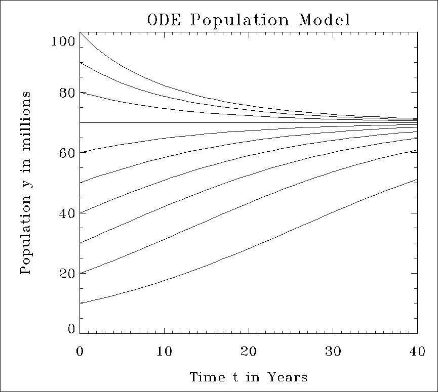
For this example, choose ε = 0.07 and σ = 0.001, and solve the ODE for various values of initial conditions. The resulting solutions are plotted. Note that the line y = 0.07/.001 = 70 is the limiting curve, regardless of the initial population value. For each initial condition, the population at time t = 40 is given.

1. Open a text editor to type this program, which you save as population_ode.pro.

2. Type or paste in the following program.

note

Comments are preceded by semicolons (;). The plus character (+) is needed when two character strings are concatenated into one. Character strings can be entered only one line at a time; therefore, any string longer than one line must be broken into two by using a plus sign to combine them. The plus sign can be placed at the end of the first line or at the beginning of the second.

; Define a function to evaluate the right-hand side of the ODE

FUNCTION ode_1, t, y

epsilon = 0.07

sigma = 0.001

RETURN, epsilon*y - sigma*y*y

END

; Main program

PRO POPULATION_ODE

; The variable t represents time in years.

t = [0, 40]

t = FINDGEN(41)

; Set up a matrix to hold the ODE solution corresponding to

; runs with 10 different initial solutions.

yprime = FLTARR(10, 41)

WINDOW, 0, XSize=875, YSize=800, XPos=3, YPos=30, $
Title='PV-WAVE ODE Integrator'

; Set up the axes for a plot of the solutions.

PLOT, yprime(0, *), t, YRange=[0, 100], XRange=[0, 40], $
/NoData, Title='!17ODE Population Model', $
XTitle='Time t in Years', $
YTitle='Population y in millions', CharSize=2

; For each solution print initial condition and final value.

PM, 'Initial Condition y(0) Population at t=40'

; Loop over 10 different initial conditions.

FOR i=10, 100, 10 DO BEGIN

yinitial = [i]

index = i/10 -1

; Call PV-WAVE IMSL Mathematics function ODE.

yprime(index,*) = ODE(t, yinitial, 'ode_1')

; Print initial and final solutions.

PRINT, yinitial(0),'      ', yprime(index, 40)

; Plot solutions.

OPLOT, t, yprime(index, *)

ENDFOR

END

3. Save the file as population_ode.pro. Now you are ready to compile and run the program.

4. Enable the mathematics and statistics functions. By default, the functions associated with PV‑WAVE IMSL Mathematics and PV‑WAVE IMSL Statistics are disabled. To enable them, if needed, enter the following:

@waveadv

5. Execute the prep_plot.pro file. It is used to reset plotting parameters and system variables:

prep_plot

note	The prep_plot.pro file is located in <RW_DIR>\docs\tutorial\code directory. If that directory is not in your path, change directories to it before running prep_plot: CD, '<RW_DIR>\docs\tutorial\code'

6. If necessary, change to the directory where you saved population_ode.pro.

7. Compile the program. Type:

.RUN population_ode

The program is compiled.

If you made a typing error, you will receive an error message. In this case, go back to your text editor and correct the mistake; save the program; then recompile the program. You do not need to close (exit) PV‑WAVE.

note	A runtime error could stop the program at a level below the main level. To return to the main program level, type RETALL at the WAVE> prompt.

8. Use the program by entering the following at the WAVE> prompt:

population_ode

The program returns the values for the Initial Condition and for the Population at each condition:

      Initial Condition y(0)

       Population at t = 40

10                   51.2446

20                   60.8025

30                   64.7429

40                   67.0317

50                   68.4430

60                   69.3272

70                   70.0000

80                   70.5622

90                   70.9890

100                  71.3117

then it plots the values as shown in Population Model Plot.

Figure 10-3: Population Model Plot

Version 2017.0