FMIN Function (PV-WAVE Advantage)
Finds the minimum point of a smooth function f (x) of a single variable using function evaluations and, optionally, through both function evaluations and first derivative evaluations.
Usage
result = FMIN(f, a, b[, grad])
Input Parameters
f—Scalar string specifying a user-supplied function to compute the value of the function to be minimized. Parameter f accepts the following parameter and returns the computed function value at this point:
 x
x—Point at which the function is to be evaluated.
a—Lower endpoint of the interval in which the minimum point of f is to be located.
b—Upper endpoint of the interval in which the minimum point of f is to be located.
grad—Scalar string specifying a user-supplied function to compute the first derivative of the function. Parameter grad accepts the following parameter and returns the computed derivative at this point:
 x
x—Point at which the derivative is to be evaluated.
Returned Value
result—The point at which a minimum value of f is found. If no value can be computed, then NaN (Not a Number) is returned.
Input Keywords
Double—If present and nonzero, double precision is used.
XGuess—Initial guess of the minimum point of f. Default: XGuess = (a + b)/2
Max_Evals—Maximum number of function evaluations allowed. Default: Max_Evals = 1000
Err_Abs—Required absolute accuracy in the final value of x. On a normal return, there are points on either side of x within a distance Err_Abs at which f is no less than f at x. Keyword Err_Abs cannot be used if the optional parameter grad is supplied. Default: Err_Abs = 0.0001
Step—Order of magnitude estimate of the required change in x. Keyword Step cannot be used if the optional parameter grad is supplied. Default: Step = 1.0
Err_Rel—Required relative accuracy in the final value of x. This is the first stopping criterion. On a normal return, the solution x is in an interval that contains a local minimum and is less than or equal to max (1.0, | x |) * Err_Rel. When the given Err_Rel is less than zero, SQRT(ε) is used as Err_Rel, where ε is the machine precision. Keyword Err_Rel can only be used if the optional parameter grad is supplied. Default: Err_Rel = SQRT(ε)
Tol_Grad—Derivative tolerance used to decide if the current point is a local minimum. This is the second stopping criterion. Parameter x is returned as a solution when grad is less than or equal to Tol_Grad. Keyword Tol_Grad should be nonnegative; otherwise, zero is used. Keyword Tol_Grad can only be used if the optional parameter grad is supplied. Default: Tol_Grad = SQRT(ε), where ε is the machine precision.
Output Keywords
FValue—Function value at point x. Keyword FValue can only be used if the optional parameter grad is supplied.
GValue—Derivative value at point x. Keyword GValue can only be used if the optional parameter grad is supplied.
Discussion
Function FMIN uses a safeguarded, quadratic interpolation method to find a minimum point of a univariate function. Both the code and the underlying algorithm are based on the subroutine ZXLSF written by M.J.D. Powell at the University of Cambridge.
The FMIN function finds the least value of a univariate function, f, which is specified by the function f. (Other required data are two points A and B that define an interval for finding a minimum point from an initial estimate of the solution, x0, where x0 = XGuess.) The algorithm begins the search by moving from x0 to x = x0 + s, where s = Step is an estimate of the required change in x and may be positive or negative. The first two function evaluations indicate the direction to the minimum point, and the search strides out along this direction until a bracket on a minimum point is found or until x reaches one of the endpoints a or b. During this stage, the step length increases by a factor of between 2 and 9 per function evaluation. The factor depends on the position of the minimum point that is predicted by quadratic interpolation of the three most recent function values.
When an interval containing a solution has been found, the three points are as follows:
x1, x2, x3, with x1 < x2 < x3, f(x1) ≥ f(x2), and f(x2) ≥ f(x3)
The following rules should be considered when choosing the new x from these three points:

the estimate of the minimum point that is given by quadratic interpolation of the three function values

a tolerance parameter
η, which depends on the closeness of |
f| to a quadratic

whether
x2 is near the center of the range between
x1 and
x3 or is relatively close to an end of this range
In outline, the value of x is as near as possible to predicted minimum point, subject to being at least ε from x2 and subject to being in the longer interval between x1 and x2 or x2 and x3, when x2 is close to x1 or x3.
The algorithm is intended to provide fast convergence when f has a positive and continuous second derivative at the minimum and to avoid gross inefficiencies in pathological cases, such as the following:
f(x) = x + 1.001 | x |
The algorithm can automatically make ε large in the pathological cases. In this case, it is usual for a new value of x to be at the midpoint of the longer interval that is adjacent to the least calculated function value. The midpoint strategy is used frequently when changes to f are dominated by computer rounding errors, which happens if the user requests an accuracy that is less than the square root of the machine precision. In such cases, the subroutine claims to have achieved the required accuracy if it decides that there is a local minimum point within distance δ of x, where δ = Err_Abs, even though the rounding errors in f may cause the existence of other local minimum points nearby. This difficulty is inevitable in minimization routines that use only function values, so high-precision arithmetic is recommended.
If parameter grad is supplied, then the FMIN function uses a descent method with either the secant method or cubic interpolation to find a minimum point of a univariate function. It starts with an initial guess and two endpoints. If any of the three points is a local minimum point and has least function value, the function terminates with a solution; otherwise, the point with least function value is used as the starting point.
From the starting point, for example xc, the function value fc = f (xc), the derivative value gc = g (xc), and a new point xn, defined by xn = xc – gc, are computed. The function fn = f (xn) and the derivative gn = g (xn) are then evaluated. If either fn ≥ f c or gn has the opposite sign of gc, then a minimum point exists between xc and xn, and an initial interval is obtained; otherwise, since xc is kept as the point that has lowest function value, an interchange between xn and xc is performed. The secant method is then used to get a new point:
Let xn <− xs. Repeat this process until an interval containing a minimum is found or one of the following convergence criteria is satisfied:
Criterion 1: | xc – xn | ≤ εc
Criterion 2: | gc | ≤ εg
where εc = max {1.0, | xc |} * ε, ε is a relative error tolerance and εg is a gradient tolerance.
When convergence is not achieved, a cubic interpolation is performed to obtain a new point. The function and derivative are then evaluated at that point; accordingly, a smaller interval that contains a minimum point is chosen. A safeguarded method is used to ensure that the interval be reduced by at least a fraction of the previous interval. Another cubic interpolation is then performed, and this function is repeated until one of the stopping criteria is met.
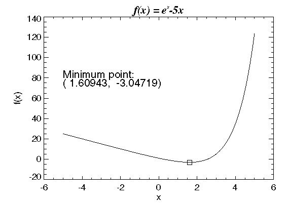
Example 1
A minimum point of
f(
x) =
ex – 5
x is found. The results are shown in
Figure 9-1: Minimum Point of a Smooth Function on page 418.
.RUN
; Define the function to be used.
FUNCTION f, x
RETURN, EXP(x) - 5 * x
END
; Call FMIN to compute the minimum.
xmin = FMIN('f', -100, 100); Print results.
PM, xmin
; PV-WAVE prints: 1.60943
x = 10 * FINDGEN(100)/99 - 5
!P.Font = 0
; Plot results.
PLOT, x, f(x), Title = '!8f(x) = e!Ex!N-5x!3', XTitle = 'x', $
YTitle = 'f(x)'
OPLOT, [xmin], [f(xmin)], Psym = 6
str = '(' + STRCOMPRESS(xmin) + ',' + STRCOMPRESS(f(xmin)) + ')'OPLOT, [xmin],[f(xmin)], Psym = 6
XYOUTS, -5, 80, 'Minimum point:!C' + str, Charsize = 1.2
Example 2
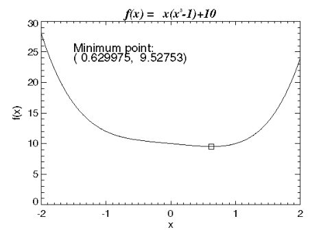
In this example, parameter
grad is supplied, and a minimum point of
f(
x) =
x (
x3 – 1 ) + 10
is found with an initial guess
x0 = 3. The results are shown in
Figure 9-2: Minimum Point of a Smooth Function on page 419.
.RUN
FUNCTION f, x
RETURN, x * (x^3 - 1) + 10
END
.RUN
FUNCTION grad, x
RETURN, 4 * x^3 - 1
END
xmin = FMIN('f', -10, 10, 'grad')x = 4 * FINDGEN(100)/99 - 2
!P.Font = 0
PLOT, x, f(x), Title = '!8f(x) = x(x!E3!N-1)+10!3', $
XTitle ='x', YTitle = 'f(x)'
OPLOT, [xmin], [f(xmin)], Psym = 6
str = '(' + STRCOMPRESS(xmin) + ',' + STRCOMPRESS(f(xmin)) + ')'XYOUTS, -1.5, 25, 'Minimum point:'+str, Charsize = 1.2
Warning Errors
MATH_MIN_AT_LOWERBOUND—Final value of x is at the lower bound.
MATH_MIN_AT_UPPERBOUND—Final value of x is at the upper bound.
MATH_MIN_AT_BOUND—Final value of x is at a bound.
MATH_NO_MORE_PROGRESS—Computer rounding errors prevent further refinement of x.
MATH_TOO_MANY_FCN_EVAL—Maximum number of function evaluations exceeded.
Version 2017.0
Copyright © 2017, Rogue Wave Software, Inc. All Rights Reserved.


