Computes a smooth bivariate interpolant to scattered data that is locally a quintic polynomial in two variables.

xydata—Two-dimensional array containing the data points for the interpolation problem. Argument xydata is dimensioned (2, N_ELEMENTS (fdata)). The ith data point (xi, yi) is stored in xydata (0, i) = xi and xydata (1, i) = yi.

fdata—One-dimensional array containing the values to be interpolated.

xout—One-dimensional array specifying the x values for the output grid. It must be strictly increasing.

yout—One-dimensional array specifying the y values for the output grid. It must be strictly increasing.

result—A two-dimensional array containing the grid of values of the interpolant.

Double—If present and nonzero, double precision is used.

SCAT2DINTERP computes a C1 interpolant to scattered data in the plane. Given the data points (in R3):

where n = N_ELEMENTS(xydata) / 2, SCAT2DINTERP returns the values of the interpolant s on the user-specified grid. The computation of s is as follows.

First, the Delaunay triangulation of the points:

is computed. On each triangle T in this triangulation, s has the following form:

Thus, s is a bivariate quintic polynomial on each triangle of the triangulation. In addition:

and s is continuously differentiable across the boundaries of neighboring triangles. These conditions do not exhaust the freedom implied by the above representation. This additional freedom is exploited in an attempt to produce an interpolant that is faithful to the global shape properties implied by the data. For more information on this procedure, refer to the article by Akima (1978). The output grid is specified by the two real vectors,  xout and yout, that represent the first (second) coordinates of the grid.

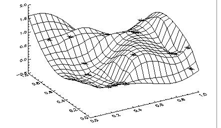
In this example, SCAT2DINTERP is used to fit a surface to randomly scattered data. The resulting surface and the original data points are then plotted as shown in Figure 4-16: Fit to Scattered Data on page 185.

RANDOMOPT, Set = 12345

ndata = 15

xydata = FLTARR(2, ndata)

xydata(*) = RANDOM(2 * ndata)

fdata = RANDOM(ndata)

x = xydata(0, *)

y = xydata(1, *)

; Define the grid used to evaluate the computed surface.

ngrid = 20

xout = FINDGEN(ngrid)/(ngrid - 1)

yout = FINDGEN(ngrid)/(ngrid - 1)

; Call SCAT2DINTERP.

surf = SCAT2DINTERP(xydata, fdata, xout, yout)

; Plot the computed surface.

SURFACE, surf, xout, yout, /Save, Ax = 45, Charsize = 1.5

; Plot the original data points.

PLOTS,  x, y, fdata, /T3d, Symsize = 2, Psym = 2

MATH_DUPLICATE_XYDATA_VALUES—Two-dimensional data values must be distinct.

MATH_XOUT_NOT_STRICTLY_INCRSING—Vector xout must be strictly increasing.

MATH_YOUT_NOT_STRICTLY_INCRSING—Vector yout must be strictly increasing.