BSKNOTS Function (PV-WAVE Advantage)
Computes the knots for a spline interpolant.
Usage
result = BSKNOTS(xdata)
Input Parameters
xdata—One-dimensional array containing the abscissas of the interpolation problem.
Returned Value
result—A one-dimensional array containing the computed knots.
Input Keywords
Double—If present and nonzero, double precision is used.
Order—Order of the spline subspace for which the knots are desired. Default: Order = 4, i.e., cubic splines
Optimum—If present and nonzero, knots that satisfy an optimal criterion are computed. See Discussion for more information.
Itmax—Integer value used to set the maximum number of iterations of Newton’s method. To use this keyword, keyword Optimum must also be set. Default: Itmax = 10
Discussion
Given the data points x = xdata, the order of the spline k = Order, and the number n = N_ELEMENTS (xdata) of elements in xdata, the default action of BSKNOTS returns a knot sequence that is appropriate for interpolation of data on x by splines of order k (the default order is k = 4). The knot sequence is contained in its n + k elements. If k is even and it is assumed that the entries in the input vector x are increasing, then the resulting knot sequence t is returned as follows:
ti = x0 for i = 0, ..., k – 1
ti = xi – k/2 – 1 for i = k, ..., n – 1 (1)
ti = xn – 1 for i = n, ..., n + k – 1
There is some discussion concerning this selection of knots in de Boor (1978, p. 211). If k is odd, then t is returned as follows:
It is not necessary to sort the values in xdata.
If keyword Optimum is set, then the knot sequence returned minimizes the constant c in the error estimate:
|| f – s || ≤ c || f (k) ||
where f is any function in Ck and s is the spline interpolant to f at the abscissa x with knot sequence t.
The algorithm is based on a routine described by de Boor (1978, p. 204), which in turn is based on a theorem of Micchelli et al. (1976).
Example 1
In this example, knots for a cubic spline are generated and printed. Notice that the knots are stacked at the endpoints; also, the second and next-to-last data points are not knots.
x = FINDGEN(6)
knots = BSKNOTS(x)
PM, knots, Format = '(f5.2)'
; PV-WAVE prints the following:
; 0.00
; 0.00
; 0.00
; 0.00
; 2.00
; 3.00
; 5.00
; 5.00
; 5.00
; 5.00
Example 2
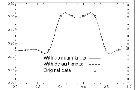
This example compares the default knots with the knots returned using keyword
Optimize as shown in
Optimum Knot Placement. The order is changed from the default value of 4 to 3.
; Define the abscissa values.
x = FINDGEN(11)/10
; Define the function values.
f = FLTARR(11)
f(0:3) = .25
f(4:7) = .5
f(8:10) = .25
; Compute the default spline.
sp1 = BSINTERP(x, f)
; Compute the optimum knots of order 3.
knots2 = BSKNOTS(x, /Optimum, Order = 3)
; Compute the spline of order 3, with the optimum knots.
sp2 = BSINTERP(x, f, XKnots = knots2, XOrder = 3)
; Evaluate the two splines for plotting.
x2 = FINDGEN(100)/99
sp1eval = SPVALUE(x2, sp1)
sp2eval = SPVALUE(x2, sp2)
; Plot the results.
PLOT, x2, sp1eval, Linestyle = 2
OPLOT, x2, sp2eval
OPLOT, x, f, Psym = 6
XYOUTS, .25, .18, 'With optimum knots:', Charsize = 1.5
OPLOT, [.65, .75], [.188, .188]
XYOUTS, .25, .135, 'With default knots:', Charsize = 1.5
OPLOT, [.65, .75], [.143, .143], Linestyle = 2
XYOUTS, .3, .09, 'Original data', Charsize = 1.5
OPLOT, [.7], [.098], Psym = 6
Warning Errors
MATH_NO_CONV_NEWTON—Newton’s method iteration did not converge.
Fatal Errors
MATH_DUPLICATE_XDATA_VALUES—The xdata values must be distinct.
MATH_ILL_COND_LIN_SYS—Interpolation matrix is singular. The xdata values may be too close together.
Version 2017.0
Copyright © 2017, Rogue Wave Software, Inc. All Rights Reserved.


