Computes a one- or two-dimensional, least-squares spline approximation.

If a one-dimensional B-spline is desired, then arguments xdata, fdata, and xspacedim are required. If a two-dimensional, tensor-product B-spline is desired, then arguments xdata, ydata, fdata, xspacedim, and yspacedim are required.

xdata—One-dimensional array containing the data points in the x-direction.

ydata—One-dimensional array containing the data points in the y-direction.

fdata—Array containing the values to be approximated. If a one-dimensional approximation is to be computed, then fdata is a one-dimensional array. If a two-dimensional approximation is to be computed, then fdata is a two-dimensional array, where fdata (i, j) contains the value at (xdata (i), ydata(j)).

xspacedim—Linear dimension of the spline subspace for the x variable. It should be smaller than the number of data points in the x-direction and greater than or equal to the order of the spline in the x-direction (whose default value is 4).

yspacedim—Linear dimension of the spline subspace for the y variable. It should be smaller than the number of data points in the y-direction and greater than or equal to the order of the spline in the y-direction (whose default value is 4).

result—A structure containing all the information to determine the spline fit.

Double—If present and nonzero, double precision is used.

XOrder—Specifies the order of the spline in the x-direction. Default: XOrder = 4, i.e., cubic splines

YOrder—Specifies the order of the spline in the y-direction. If a one-dimensional spline is being computed, then YOrder has no effect on the computations. Default: YOrder = 4, i.e., cubic splines

XKnots—Specifies the array of knots in the x-direction to be used when computing the definition of the spline. Default: knots are equally spaced in the x-direction

YKnots—Specifies the array of knots in the y-direction to be used when computing the definition of the spline. Default: knots are equally spaced in the y-direction

XWeights—Array containing the weights to use in the x‑direction. Default: all weights equal to 1

YWeights—Array containing the weights to use in the y‑direction. If a one-dimensional spline is being computed, then YWeights has no effect on the computations. Default: all weights equal to 1

Optimize—If present and nonzero, optimizes the knot locations by attempting to minimize the least-squares error as a function of the knots. This keyword is only active if a one-dimensional spline is being computed.

Sse—Specifies the named variable into which the weighted error sum of squares is stored.

Function BSLSQ computes a least-squares approximation to weighted data returning either a one-dimensional B-spline or a two-dimensional, tensor-product B-spline. The determination of whether to return a one- or two-dimensional spline is made based on the number of arguments passed to the function.

Make the following identifications:

For convenience, assume that the sequence x is increasing (although the function does not require this).

By default, k = 4 and the knot sequence selected equally distributes the knots through the distinct xi’s. In particular, the m + k knots are generated in [x0, xn – 1 ] with k knots stacked at each of the extreme values. The interior knots are equally spaced in the interval.

Once knots t and weights w are determined (and assuming that keyword Optimize is not set), then the function computes the spline least-squares fit to the data by minimizing over the linear coefficients aj, such that:

where Bj, j = 0, ..., m – 1, is a (B-spline) basis for the spline subspace.

The XOrder keyword allows the user to choose the order of the spline fit. The XKnots keyword allows user specification of knots. The one-dimensional functionality of BSLSQ is based on the routine L2APPR by de Boor (1978, p. 255).

If Optimize is chosen, the function attempts to find the best placement of knots that minimizes the least-squares error to the given data by a spline of order k with m coefficients. For this problem, it is necessary that m > k. Then, to find the minimum of the functional, use the following:

The technique employed here uses the fact that for a fixed-knot sequence t the minimization in a is a linear least-squares problem that is easily solved. Thus, objective function F is a function of only t by setting the following:

A Gauss-Seidel (cyclic coordinate) method is then used to reduce the value of the new objective function G. In addition to this local method, there is a global heuristic built into the algorithm that is useful if the data arise from a smooth function. This heuristic is based on the routine NEWNOT of de Boor (1978, pp. 184, 258–261).

The guess, tg, for the knot sequence is either provided by the user or is the default. This must be a valid knot sequence for splines of order k with:

with tg nondecreasing and tgi < tgi + k for i = 0, ..., m – 1.

In regard to execution speed, this function can be several orders of magnitude slower than a simple least-squares fit.

The return value for this function is a structure containing all the information to determine the spline (stored in B-spline form) that is computed by this function.

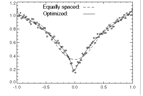
In Two Fits to Noisy SQRT( |x| ), two cubic splines are fit to SQRT( |x| ). Both splines are cubics with the same xspacedim = 8. The first spline is computed with the default settings, while the second spline is computed by optimizing the knot locations using the Optimize keyword.

If a two-dimensional, tensor-product B-spline is desired, the BSLSQ function computes a tensor‑product spline, least-squares approximation to weighted, tensor-product data. The input for this function consists of data vectors to specify the tensor-product grid for the data, two vectors with the weights (optional, the default is 1), the values of the surface on the grid, and the specification for the tensor-product spline (optional, a default is chosen). The grid is specified by the two vectors x = xdata and y = ydata of length n = N_ELEMENTS(xdata) and m= N_ELEMENTS(ydata), respectively. A two-dimensional array f = fdata contains the data values to be fit. The two vectors wx = XWeights and wy = YWeights contain the weights for the weighted, least-squares problem. The information for the approximating tensor-product spline can be provided using keywords XOrder, YOrder, XKnots, and YKnots. This information is contained in kx = XOrder, tx = XKnots, and n = xspacedim for the spline in the first variable, and in ky = YOrder, ty = YKnots, and m = yspacedim for the spline in the second variable.

This function computes coefficients for the tensor-product spline by solving the normal equations in tensor-product form as discussed in de Boor (1978, Chapter 17). For more information, see the paper by Grosse (1980).

As the computation proceeds, coefficients c are obtained minimizing:

where the function Bkl is the tensor-product of two B-splines of order kx and ky:

The spline:

and its partial derivatives can be evaluated using the SPVALUE Function (PV-WAVE Advantage).

The return value for this function is a structure containing all the information to determine the spline that is computed by this function. For example, the following code sequence evaluates this spline (stored in the structure sp) at (x, y) and returns the value in v:

v = SPVALUE(x, y, sp)

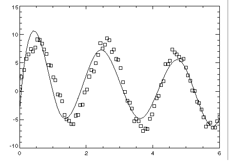
This example fits data generated from a trigonometric polynomial:

where ε is a random uniform deviate over the range [–1, 1]. The data is obtained by evaluating this function at 90 equally spaced points on the interval [0, 6]. This data is fit with a cubic spline with 12 degrees of freedom (eight equally spaced interior knots). The computed fit and original data are then plotted, as shown in One-Dimensional Least-Squares B-Spline Fit, as follows:

; Set up the data.

n = 90

x = 6 * FINDGEN(n)/(n - 1)

f = 1 + SIN(x) + 7 * SIN(3 * x) + (1 - 2 * RANDOM(n))

; Compute the spline fit.

sp = BSLSQ(x, f, 8)

; Evaluate the computed spline at the original data abscissa.

speval = SPVALUE(x, sp)

; Plot the results.

PLOT, x, speval

OPLOT, x, f, Psym = 6

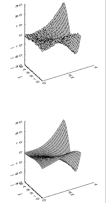
This example fits noisy data that arises from the function exsin (x + y) + ε, where ε is a random uniform deviate in the range (–1, 1), on the rectangle [0, 3] × [0, 5]. This function is sampled on a 50 × 25 grid and the original data and the evaluations of the computed spline are plotted as shown in Two-Dimensional B-Spline Fit to Noisy Data.

; Generate noisy data on a 50 by 25 grid.

nx = 50

ny = 25

x = 3 * FINDGEN(nx)/(nx - 1)

y = 5 * FINDGEN(ny)/(ny - 1)

f = FLTARR(nx, ny)

FOR i=0L, nx - 1 DO f(i, *) = EXP(x(i)) * $

   SIN(x(i) + y) + 2 * RANDOM(ny) - 1

; Call BSLSQ to compute the least-squares fit. Notice that 

; xspacedim = 5 and yspacedim = 7.

sp = BSLSQ(x, y, f, 5, 7)

; Evaluate the fit on the original grid.

speval = SPVALUE(x, y, sp)

; Plot the original data and the fit in the same window.

!P.Multi = [0, 1, 2]

WINDOW, XSize = 500, YSize = 800

SURFACE, f, x, y, Ax = 45, XTitle = 'X', YTitle = 'Y'

SURFACE, speval, x, y, Ax = 45, XTitle = 'X', YTitle = 'Y'

MATH_ILL_COND_LSQ_PROB—Least-squares matrix is ill‑conditioned. Solution might not be accurate.

MATH_SPLINE_LOW_ACCURACY—There may be less than one digit of accuracy in the least-squares fit. Try using higher precision if possible.

MATH_OPT_KNOTS_STACKED_1—Knots found to be optimal are stacked more than Order. This indicates that fewer knots will produce the same error sum of squares. Knots have been separated slightly.

MATH_KNOT_MULTIPLICITY—Multiplicity of the knots cannot exceed the order of the spline.

MATH_KNOT_NOT_INCREASING—Knots must be nondecreasing.

MATH_SPLINE_LRGST_ELEMNT—Data arrays xdata and ydata must satisfy datai ≤ tSpline_Space_Dim, for i = 1, ..., num_data.

MATH_SPLINE_SMLST_ELEMNT—Data arrays xdata and ydata must satisfy datai ≥ tOrder – 1, for i = 1, ..., num_data.

MATH_NEGATIVE_WEIGHTS—All weights must be greater than or equal to zero.

MATH_DATA_DECREASING—The xdata values must be nondecreasing.

MATH_XDATA_TOO_LARGE—Array xdata must satisfy xdatai ≤ tndata, for i = 1, ..., ndata.

MATH_XDATA_TOO_SMALL—Array xdata must satisfy xdatai ≥ tOrder – 1, for i = 1, ..., ndata.

MATH_OPT_KNOTS_STACKED_2—Knots found to be optimal are stacked more than Order. This indicates fewer knots will produce the same error sum of squares.