MLFF_NETWORK_FORECAST Function (PV-WAVE Advantage)
Calculates forecasts for trained multilayered feedforward neural networks.
Usage
result = MLFF_NETWORK_FORECAST(network, categorical, continuous)
Input Parameters
network—Structure containing the trained feedforward network. See the
MLFF_NETWORK Function (PV-WAVE Advantage).
categorical—Array of size n_categorical containing the categorical input variables, where n_categorical indicates the number of categorical attributes. If there are no categorical variables, set categorical equal to the scalar value of 0.
continuous—Array of size n_continuous containing the continuous input variables, where n_continuous indicates the number of continous attributes. If there are no continuous variables, set continuous equal to the scalar value of 0.
Returned Value
result—Array of size n_outputs containing the forecasts, where n_outputs is the number of output perceptrons in the network. n_outputs = network.layers(network.n_layers-1).n_nodes.
Discussion
For further information, refer to the Discussion section of the
MLFF_NETWORK_TRAINER Function (PV-WAVE Advantage).
Example
This example trains a two-layer network using 90 training patterns from one nominal and one continuous input attribute. The nominal attribute has three classifications which are encoded using binary encoding. This results in three binary network input columns. The continuous input attribute is scaled to fall in the interval [0,1].
The network training targets were generated using the relationship:
Y = 10*X1 + 20*X2 + 30*X3 + 2.0*X4
where X1, X2, X3 are the three binary columns, corresponding to the categories 1-3 of the nominal attribute, and X4 is the scaled continuous attribute.
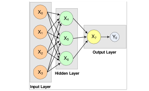
The structure of the network consists of four input nodes and two layers, with three perceptrons in the hidden layer and one in the output layer.
A 2-layer, Feedforward Network with 4 Inputs and 1 Output illustrates this structure:
There are a total of 15 weights and 4 bias weights in this network. In the output below, 19 weight values are printed. Weights 0–14 correspond to the links between the network nodes. Weights 15–18 correspond to the bias values associated with the four non-input layer nodes, X4, X5, X6, and X7.
There are a total of 100 outputs. Training the first 90 and forecasting the 10 and compare the forecasted values with the actual outputs.
n_obs = 100
n_cat = 3
n_cont = 1
categorical = [ $
1, 0, 0, 1, 0, 0, 1, 0, 0, 1, 0, 0, 1, 0, 0, 1, 0, 0, 1, 0, $
0, 1, 0, 0, 1, 0, 0, 1, 0, 0, 1, 0, 0, 1, 0, 0, 1, 0, 0, 1, $
0, 0, 1, 0, 0, 1, 0, 0, 1, 0, 0, 1, 0, 0, 1, 0, 0, 1, 0, 0, $
1, 0, 0, 1, 0, 0, 1, 0, 0, 1, 0, 0, 1, 0, 0, 1, 0, 0, 1, 0, $
0, 1, 0, 0, 1, 0, 0, 1, 0, 0, 1, 0, 0, 1, 0, 0, 1, 0, 0, 1, $
0, 0, 1, 0, 0, 0, 1, 0, 0, 1, 0, 0, 1, 0, 0, 1, 0, 0, 1, 0, $
0, 1, 0, 0, 1, 0, 0, 1, 0, 0, 1, 0, 0, 1, 0, 0, 1, 0, 0, 1, $
0, 0, 1, 0, 0, 1, 0, 0, 1, 0, 0, 1, 0, 0, 1, 0, 0, 1, 0, 0, $
1, 0, 0, 1, 0, 0, 1, 0, 0, 1, 0, 0, 1, 0, 0, 1, 0, 0, 1, 0, $
0, 1, 0, 0, 1, 0, 0, 1, 0, 0, 1, 0, 0, 1, 0, 0, 0, 1, 0, 0, $
1, 0, 0, 1, 0, 0, 1, 0, 0, 1, 0, 0, 1, 0, 0, 1, 0, 0, 1, 0, $
0, 1, 0, 0, 1, 0, 0, 1, 0, 0, 1, 0, 0, 1, 0, 0, 1, 0, 0, 1, $
0, 0, 1, 0, 0, 1, 0, 0, 1, 0, 0, 1, 0, 0, 1, 0, 0, 1, 0, 0, $
1, 0, 0, 1, 0, 0, 1, 0, 0, 1, 0, 0, 1, 0, 0, 1, 0, 0, 1, 0, $
0, 1, 0, 0, 1, 0, 0, 1, 0, 0, 1, 0, 0, 1, 0, 0, 1, 0, 0, 1]
; Reform the categorical array to be 2D (three columns
; corresponding to the three categorical variables, 100
; observations each.
categorical = TRANSPOSE(REFORM(categorical, 3,100))
continuous = [ $
4.007054658, 7.10028447, 4.740350984, 5.714553211, $
6.205437459, 2.598930065, 8.65089967, 5.705787357, $
2.513348184, 2.723795955, 4.1829356, 1.93280416, $
0.332941608, 6.745567628, 5.593588463, 7.273544478, $
3.162117939, 4.205381208, 0.16414745, 2.883418275, $
0.629342241, 1.082223406, 8.180324708, 8.004894314, $
7.856215418, 7.797143157, 8.350033996, 3.778254431, $
6.964837082, 6.13938006, 0.48610387, 5.686627923, $
8.146173848, 5.879852653, 4.587492779, 0.714028533, $
7.56324211, 8.406012623, 4.225261454, 6.369220241, $
4.432772218, 9.52166984, 7.935791508, 4.557155333, $
7.976015058, 4.913538616, 1.473658514, 2.592338905, $
1.386872932, 7.046051685, 1.432128376, 1.153580985, $
5.6561491, 3.31163251, 4.648324851, 5.042514515, $
0.657054195, 7.958308093, 7.557870384, 7.901990083, $
5.2363088, 6.95582150, 8.362167045, 4.875903563, $
1.729229471, 4.380370223, 8.527875685, 2.489198107, $
3.711472959, 4.17692681, 5.844828801, 4.825754155, $
5.642267843, 5.339937786, 4.440813223, 1.615143829, $
7.542969339, 8.100542684, 0.98625265, 4.744819569, $
8.926039258, 8.813441887, 7.749383991, 6.551841576, $
8.637046998, 4.560281415, 1.386055087, 0.778869034, $
3.883379045, 2.364501589, 9.648737525, 1.21754765, $
3.908879368, 4.253313879, 9.31189696, 3.811953836, $
5.78471629, 3.414486452, 9.345413015, 1.024053777]
output = [ $
18.01410932, 24.20056894, 19.48070197, 21.42910642, $
22.41087492, 15.19786013, 27.30179934, 21.41157471, $
15.02669637, 15.44759191, 18.3658712, 13.86560832, $
10.66588322, 23.49113526, 21.18717693, 24.54708896, $
16.32423588, 18.41076242, 10.3282949, 15.76683655, $
11.25868448, 12.16444681, 26.36064942, 26.00978863, $
25.71243084, 25.59428631, 26.70006799, 17.55650886, $
23.92967416, 22.27876012, 10.97220774, 21.37325585, $
26.2923477, 21.75970531, 19.17498556, 21.42805707, $
35.12648422, 36.81202525, 28.45052291, 32.73844048, $
28.86554444, 39.04333968, 35.87158302, 29.11431067, $
35.95203012, 29.82707723, 22.94731703, 25.18467781, $
22.77374586, 34.09210337, 22.86425675, 22.30716197, $
31.3122982, 26.62326502, 29.2966497, 30.08502903, $
21.31410839, 35.91661619, 35.11574077, 35.80398017, $
30.4726176, 33.91164302, 36.72433409, 29.75180713, $
23.45845894, 38.76074045, 47.05575137, 34.97839621, $
37.42294592, 38.35385362, 41.6896576, 39.65150831, $
41.28453569, 40.67987557, 38.88162645, 33.23028766, $
45.08593868, 46.20108537, 31.9725053, 39.48963914, $
47.85207852, 47.62688377, 45.49876798, 43.10368315, $
47.274094, 39.1205628, 32.77211017, 31.55773807, $
37.76675809, 34.72900318, 49.29747505, 32.4350953, $
37.81775874, 38.50662776, 48.62379392, 37.62390767, $
41.56943258, 36.8289729, 48.69082603, 32.04810755]
scalecont = SCALE_FILTER(continuous, 1, $
Scale_Limits=[0.0, 10.0, 0.0, 1.0])
ff_net = MLFF_NETWORK_INIT(4, 1)
ff_net = MLFF_NETWORK(ff_net, Create_hidden_layer=3)
ff_net = MLFF_NETWORK(ff_net, /Link_all, $
Weights=[REPLICATE(0.25, 12), REPLICATE(0.33, 3)])
RANDOMOPT, Set=12345
stats = MLFF_NETWORK_TRAINER(ff_net, $
categorical(0:89, *), $
scalecont(0:89), $
output(0:89), $
/Print)
PM, ff_net.nodes(0).bias, $ ;;should be 0
ff_net.nodes(1).bias, $ ;;should be 0
ff_net.nodes(2).bias, $ ;;should be 0
ff_net.nodes(3).bias ;;should be 0
; 0.000000 0.000000 0.000000 0.000000
PM, ff_net.nodes(4).bias, $ ;;should = weight[15]
ff_net.nodes(5).bias, $ ;;should = weight[16]
ff_net.nodes(6).bias, $ ;;should = weight[17]
ff_net.nodes(7).bias ;;should = weight[18]
; -43.6713 -1.25058 0.557620 -42.1712
PRINT, 'Error sum of squares at the optimum: ', stats(0)
PRINT, 'Total number of Stage I iterations: ', stats(1)
PRINT, 'Smallest error sum of squares after Stage I' + $
' training: ', stats(2)
PRINT, 'Total number of Stage II iterations: ', stats(3)
PRINT, 'Smallest error sum of squares after Stage II' + $
' training: ', stats(4)
PRINT
predictions = FLTARR(10)
FOR i=90L, 99 DO BEGIN & $
continuousObs = [scalecont(i)] & $
categoricalObs = REFORM(categorical(i,*)) & $
forecast = MLFF_NETWORK_FORECAST(ff_net, $
categoricalObs, $
continuousObs) & $
predictions(i-90) = forecast(0) & $
ENDFOR
PM, [ [output(90:99)], [predictions], $
[output(90:99)-predictions] ], $
Title='Actual vs Forecasts, and Residuals...'
Output
TRAINING PARAMETERS:
Stage II Opt. = 1
n_epochs = 15
epoch_size = 90
max_itn = 1000
max_fcn = 400
max_step = 1000.000000
rfcn_tol = 2.42218e-005
grad_tol = 0.000345267
tolerance = 0.100000
STAGE I TRAINING STARTING
Stage I: Epoch 1 - Epoch Error SS = 468.918 (Iterations=60)
Stage I: Epoch 2 - Epoch Error SS = 1421.62 (Iterations=48)
Stage I: Epoch 3 - Epoch Error SS = 468.918 (Iterations=45)
Stage I: Epoch 4 - Epoch Error SS = 884.207 (Iterations=45)
Stage I: Epoch 5 - Epoch Error SS = 468.919 (Iterations=48)
Stage I: Epoch 6 - Epoch Error SS = 4.4077e-005 (Iterations=501)
Stage I Training Converged at Epoch = 6
STAGE I FINAL ERROR SS = 0.000044
OPTIMUM WEIGHTS AFTER STAGE I TRAINING:
weight[0] = -68.5556 weight[1] = -6.88944 weight[2] = 31.8535
weight[3] = 6.46488 weight[4] = -1.08123 weight[5] = -0.555641
weight[6] = -0.031482 weight[7] = 1.05059 weight[8] = -0.0437371
weight[9] = 0.391523 weight[10] = 0.827833 weight[11] = 0.870813
weight[12] = 38.4183 weight[13] = 52.6387 weight[14] = 75.9349
weight[15] = -43.6713 weight[16] = -1.25058 weight[17] = 0.55762
weight[18] = -42.1712
STAGE I TRAINING CONVERGED
STAGE I ERROR SS = 0.000044
GRADIENT AT THE OPTIMUM WEIGHTS
g[0] = 0.000000 weight[0] = -68.555618
g[1] = 0.000000 weight[1] = -6.889442
g[2] = -0.000107 weight[2] = 31.853479
g[3] = -0.000065 weight[3] = 6.464885
g[4] = 0.015193 weight[4] = -1.081228
g[5] = -0.012458 weight[5] = -0.555641
g[6] = -0.029329 weight[6] = -0.031482
g[7] = -0.024073 weight[7] = 1.050592
g[8] = 0.042926 weight[8] = -0.043737
g[9] = -0.012146 weight[9] = 0.391523
g[10] = -0.019861 weight[10] = 0.827833
g[11] = -0.009384 weight[11] = 0.870813
g[12] = -0.000003 weight[12] = 38.418285
g[13] = -0.000886 weight[13] = 52.638702
g[14] = -0.001305 weight[14] = 75.934929
g[15] = -0.000107 weight[15] = -43.671253
g[16] = -0.026594 weight[16] = -1.250582
g[17] = 0.010919 weight[17] = 0.557620
g[18] = -0.000972 weight[18] = -42.171177
Training Completed
Error sum of squares at the optimum: 0.319787
Total number of Stage I iterations: 7.00000
Smallest error sum of squares after Stage I training: 1 825.62
Total number of Stage II iterations: 0.000000
Smallest error sum of squares after Stage II training: 1.#QNAN
Actual vs Forecasts, and Residuals...
49.2975 49.3156 -0.0180969
32.4351 32.4343 0.000782013
37.8178 37.8185 -0.000713348
38.5066 38.5075 -0.000896454
48.6238 48.6328 -0.00904846
37.6239 37.6246 -0.000656128
41.5694 41.5697 -0.000289917
36.8290 36.8293 -0.000362396
48.6908 48.7006 -0.00979614
32.0481 32.0474 0.000747681
Version 2017.0
Copyright © 2017, Rogue Wave Software, Inc. All Rights Reserved.

