QMF Procedure
Applies a perfect reconstruction quadrature mirror filter (QMF) structure to a data sequence.
Usage
QMF, h, x, n, x0, x1
QMF, h, y, n, x0, x1, /Backward
Input Parameters
h—A finite impulse response (FIR) quadrature mirror filter structure. Parameters for the forward QMF computation (default):
x—A data sequence to be processed.
n—(scalar) The length of the data sequence to process.
Parameters for the backward QMF computation:
x0—The lowpass filtered and decimated signal.
x1—The highpass filtered and decimated signal.
n—(scalar) The length of the reconstructed data sequence.
Output Parameters
Specific to the forward QMF computation (default):
x0—The filtered and decimated lowpass signal.
x1—The filtered and decimated highpass signal.
Specific to the backward QMF computation:
y—The reconstructed data sequence.
Keywords
Backward—If present and nonzero, the backward QMF operation is computed.
Discussion
QMF realizes the filter structures shown in Signal Flows for Forward and Backward QMF Procedures. The definitions of the multirate filtering operations shown in the figure are in the reference pages for FILTUP and FILTDOWN.
|
|
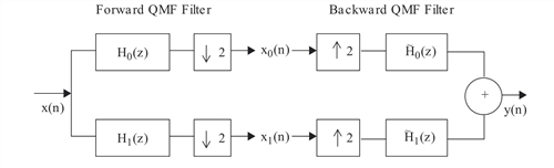
The four FIR filters shown in Signal Flows for Forward and Backward QMF Procedures are obtained from a single QMF filter that satisfies:
|H(z)|2 + |H(–z)|2 = 1
Such a QMF may be obtained using QMFDESIGN. The four filters are given by:
H0(z) = 21/2H(z)
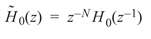
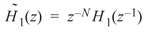
H1(z) = z–NH0(–z–1)
where N is the order of H(z). The filter H0(z) is generally a lowpass filter, and H1(z) is generally a highpass filter.
The forward QMF computation (default) uses the first half of the figure Signal Flows for Forward and Backward QMF Procedures. A QMF filter H(z) and an input signal x are used to compute the two output signals x0(n) and x1(n). The backward QMF computation uses the second half of the figure Signal Flows for Forward and Backward QMF Procedures. The backward, or inverse operation uses a QMF filter H(z) and two input signals x0(n) and x1(n) to compute the output signal y(n).
|
Note: |
QMF does not verify that the filter passed to it is actually a perfect reconstruction QMF. However, if the filter was created using QMFDESIGN and the Caution note on QMFDESIGN Function in the Discussion is followed, the filter will be a perfect reconstruction. |
Example
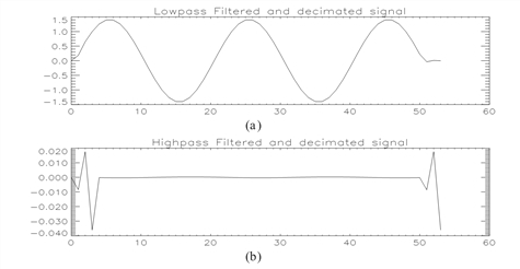
This example illustrates how a QMF is designed and then applied to a simple sine wave signal. The results are shown in Frequency Response of Quadrature Mirror Filter and Frequency Response of Quadrature Mirror Filter. The original signal is forward processed with the QMF to produce (a) x0(n), the lowpass filtered and decimated signal, and (b) x1(n), the highpass filtered and decimated signal.
k = [1, 4, 6, 4, 1]
h = QMFDESIGN(k)
hf = FREQRESP_Z(h, Outfreq = f)
; Plot the designed QMF.
PLOT, f, ABS(hf), Title = 'Quadrature Mirror Filter', $
XTitle = 'Frequency', YTitle = 'Magnitude'
; Generate a test signal.
x = SIN(0.05*!Pi*FINDGEN(100))
n = N_ELEMENTS(x)
; Forward QMF operation.
QMF, h, x, n, x0, x1
!P.Multi = [0, 1, 2]
; Plot the output signals.
PLOT, x0, Title = 'Lowpass filtered and decimated signal'
PLOT, x1, Title = 'Highpass filtered and decimated signal'
; Backward QMF operation.
QMF, h, y, n, x0, x1, /Backward
PM, MAX(ABS(x-y)), Title = 'Maximum Reconstruction Error'
; PV-WAVE prints the following:
; Maximum Reconstruction Error
; 4.4408921e-15
|
|
See Also
For Additional Information
Akansu and Haddad, 1992. Vaidyanathan, 1993.


