FIRLS Function
Approximates a deterministic frequency-domain or statistical time-domain, least-squares, linear-phase finite impulse response (FIR) filter.
Usage
result = FIRLS(n, f, amplitude)
result = FIRLS(n, rss, rnn, /Wiener)
Input Parameters
n—The length of the desired FIR filter.
f—An array of frequency points between 0.0 and 1.0.
amplitude—The desired filter amplitude response at the frequency points specified by f. Amplitude values may be positive or negative.
rss—The autocorrelation sequence of the signal.
rnn—The autocorrelation sequence of the noise.
Returned Value
result—A filter structure containing the FIR filter approximation.
Keywords
Freqsample—If present and nonzero, approximates a linear phase FIR filter using frequency domain least-squares techniques.
Interpfactor—An integer value specifying a factor by which the frequency samples are interpolated. The total number of interpolation points is given by Interpfactor*n. (Default: 4)
Oddsymm—If present and nonzero, the FIR filter approximated using deterministic frequency domain techniques will have odd symmetry.
Wiener—If present and nonzero, an odd length, even symmetric, linear phase FIR filter is approximated using statistical time domain least-squares (Wiener) techniques.
Discussion
When the keyword Freqsample is specified, FIRLS produces linear phase filters that approximate a desired amplitude frequency response. Four types of linear phase FIR filters can be approximated. They are:
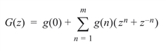
Type 1 filters have odd length n = 2m + 1, even symmetry, and are given by:
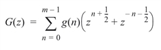
Type 2 filters have even length n = 2m, even symmetry, and are given by:
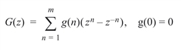
Type 3 filters have odd length n = 2m + 1, odd symmetry, and are given by:
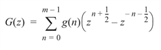
Type 4 filters have even length n = 2m, odd symmetry, and are given by:
The different types of filters are chosen by selecting the length n to be odd or even and by setting the keyword Oddsymm.
FIRLS requires the specification of a selection of distinct frequency points between 0 and 1 in increasing order:
f = [f0, f1, ... , fL]
and the desired frequency amplitude responses:
amplitude = [G(z0), G(z1), ... , G(zL)]
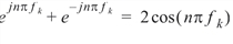
at these frequency points where:

The algorithm used to design a Type 1 linear phase filter takes the specified frequency and amplitude points and then forms a matrix A, with the k, n element given by:
and an array b with the elements of the desired frequency amplitude responses. The equation Ax = b is then solved for the array x, which contains the filter coefficients g(n), n = 0, 1, 2, ..., m. The other three types of filters are obtained in an identical manner, except the elements of the matrix A are changed appropriately.
The solution to the matrix equation depends upon the number of frequency sample points provided. If a filter of the length n has L frequency points specified and the filter has m = (n – 1)/2 distinct coefficients for n odd (or m = n/2 for n even), then the different solutions are enumerated as follows.
For the case when n is odd and the desired filter has even symmetry, FIRLS returns the following solutions:
If L – 1 > m, result is a least-squares FIR filter obtained using the specified frequency and amplitude points.
If L – 1 = m, result is the solution to the trigonometric polynomial interpolation problem.
If L – 1 < m, the frequency samples are linearly interpolated onto a uniform grid of 4*n points, and result is a least-squares FIR filter based on the interpolated frequency points.
For all other cases, FIRLS returns the following solutions:
If L > m, result is a least-squares FIR filter obtained using the specified frequency and amplitude points.
If L = m, result is the solution to the trigonometric polynomial interpolation problem.
If L < m, the frequency samples are linearly interpolated onto a uniform grid of 4*n points, and result is a least-squares FIR filter based on the interpolated frequency points.
If Interpfactor is specified, the default solutions are overridden and the frequency samples are linearly interpolated onto a uniform grid of Interpfactor*n points. The least squares solution based on the interpolated frequency points determines the filter coefficients.
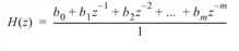
The coefficients of the four types of linear phase FIR filters are related to the coefficients of the returned filter:
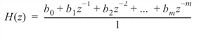
as H(z) = z–nG(z), where m = n – 1.
Further details of the equations used in the solution can be found in Parks and Burrus, 1987, sections 7.4 and 7.5.
|
Note: |
FIR filters do not have an approximation problem equivalent to the time-domain least squares problem for IIR filters (see the IIRLS Discussion section). However, a time-domain statistical least-squares approximation problem does exist for FIR filters which are solved by FIRLS. |
When Wiener is specified, FIRLS designs an optimal Type 1 linear phase FIR filter for estimating the signal s(k) from the noise corrupted observation:
x(k) = s(k) + n(k)
It is assumed that the signal and noise are stationary, have zero mean and have the known autocorrelation sequences:
rss(k) = E[s(l)s(l + k)] , k = 0, ..., m
rnn(k) = E[n(l)n(l + k)] , k = 0, ..., m
where E is the mathematical expectation operator.
The coefficients of the FIR filter:
are chosen to minimize the error:
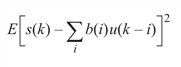
subject to the constraint that the number of coefficients is odd and the filter has linear phase.
The solution to this problem is obtained by solving the following linear equation:
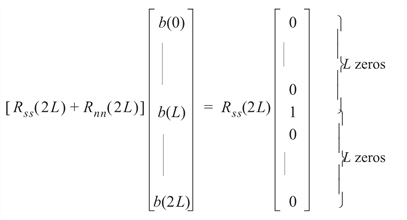
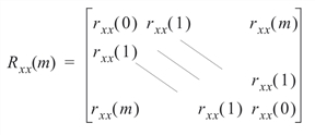
where the filter length n = 2L + 1 and the matrices Rss and Rnn are Toeplitz, defined by:
Example 1
In this example, a Type 1 FIR filter is designed to interpolate a given set of frequency amplitude points.
; Design an FIR filter.
h1 = FIRDESIGN(11,0.5,/Lowpass)
PARSEFILT, h1, name, numer1, denom1
PM, numer1, Title = 'Original FIR Filter Coefficients'
f = FINDGEN(5)/5.0
; Compute frequency response of filter at several points where
; the amplitude response is known to be positive.
desired_amplitude = ABS(FREQRESP_Z(h1, Infreq = f))
; Design FIR filter to interpolate the desired amplitude values.
h2 = FIRLS(11, f, desired_amplitude, /Freqsample)
PARSEFILT, h2, name, numer2, denom2
PM, numer2, Title = 'Interpolating FIR Filter Coefficients'
Example 2
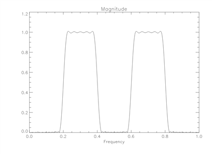
This example illustrates how to design a multiple bandpass filter using FIRLS and specified transition bands. The results are shown in Magnitude Plot of Multiple Bandpass Filter Frequency Response.
; Specify desired frequency response with transition bands.
f = [0, .18, .2, .22, .38, .4, .42, .58, .6, .62, .78, .8, .82, 1]
ampl = [0, 0, .5, 1, 1, .5, 0, 0, .5, 1, 1, .5, 0, 0]
; Design least-squares filter to approximate desired response.
h = FIRLS(101, f, ampl, /Freqsample)
hf = FREQRESP_Z(h, Outfreq = f)
; Plot the magnitude of the filter frequency response.
PLOT, f, ABS(hf), Title = 'Magnitude', XTitle = 'Frequency'
|
|
Example 3
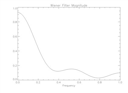
This example illustrates the use of FIRLS with the keyword Wiener to design a statistical least-squares linear phase FIR filter. The results are shown in Magnitude Plot of Wiener Filter Frequency Response.
; Covariance for first order autoregressive signal.
rss = [1, .9, .9^2, .9^3, .9^4, .9^5, .9^6, .9^7, .9^8]
; Covariance for white noise with variance 0.8.
rnn = [.8, 0, 0, 0, 0, 0, 0, 0, 0]
; Compute the Wiener filter coefficients.
h = FIRLS(9, rss, rnn, /Wiener)
hf = FREQRESP_Z(h, Outfreq = f)
; Plot the magnitude of the frequency response.
PLOT, f, ABS(hf), Title = 'Wiener Filter Magnitude', $
XTitle = 'Frequency'
|
|
See Also
For Additional Information
Parks and Burrus, 1987.
Roberts and Mullis, 1987.


