TS_OUTLIER_FORECAST Function
Computes forecasts, their associated probability limits and y weights for an outlier contaminated time series whose underlying outlier free series follows a general seasonal or nonseasonal ARMA model.
Usage
result = TS_OUTLIER_FORECAST(series, outlier_statistics, omega, delta, model, parameters, n_predict)
Input Parameters
series—An array of length n_obs by 2 containing the outlier free time series in its first column and the residuals of the series in the second column. Where n_obs is the number of observations in the time series.
outlier_statistics—Array of length num_outliers by 2 containing the outlier statistics from TS_OUTLIER_IDENTIFICATION. Where num_outliers is the number of detected outliers in the original outlier contaminated series. If num_outliers = 0, this array is ignored.
omega—Array of length num_outliers containing the y weights for the outliers determined in TS_OUTLIER_IDENTIFICATION. If num_outliers = 0, this array is ignored.
delta—The dynamic dampening effect parameter used in the outlier detection.
model—Four element array containing the numbers p, q, s, d of the ARIMA 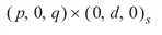 , model the outlier free series is following.
parameters—Array of length 1 + p + q containing the estimated constant, AR and MA parameters as output from TS_OUTLIER_IDENTIFICATION.
n_predict—Maximum lead time for forecasts. The forecasts are taken at origin t = n_obs, the time point of the last observed value, for lead times 1, 2, ..., n_predict.
Returned Value
result—Array of length n_predict by 3. The first column contains the forecasted values for the original outlier contaminated series. The second column contains the deviations from each forecast for computing confidence probability limits, and the third column contains the y weights of the infinite moving average form of the model.
Input Keywords
Double—If present and nonzero, double precision is used.
Confidence—Value in the exclusive interval (0, 100) used to specify the confidence percent probability limits of the forecast. Typical choices for Confidence are 90.0, 95.0 and 99.0. Default: Confidence = 95.0.
Output Keywords
Out_free_forecast—Array of length n_predict × 3 containing the forecasts for the original outlier free series in column 1, deviations from each forecast in column 2 and the y weights of the infinite moving average form of the model in column 3.
Discussion
Consider the following model for a given outlier contaminated univariate time series  :
:
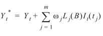
For an explanation of the notation, see the Discussion section for TS_OUTLIER_IDENTIFICATION. It follows from the formula above that the Box-Jenkins forecast at origin t for lead time l,  , can be computed as:
Therefore, computation of the forecasts for  is done in two steps:
Step 1
Compute the forecasts for the outlier free series {Yt}.
Since:
f (B)(Yt – m ) = q (B)at
where:
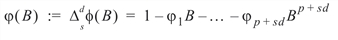
the Box-Jenkins forecast at origin t for lead time l,  , can be computed recursively as:
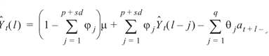
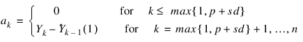
Here:

and:
Step 2
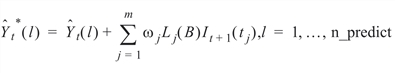
Computation of the forecasts for the original series  by adding the multiple outlier effects to the forecasts for {Yt}.
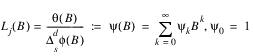
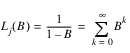
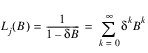
The formulas for Lj(B) for the different types of outliers are shown in Formulas for Different Types of Outliers:
|
Outlier |
Formula |
|---|---|
|
Innovational outliers (IO) |
|
|
Additive outliers (AO) |
Lj(B) = 1 |
|
Level shifts (LS) |
|
|
Temporary changes (TC) |
|
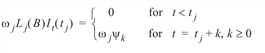
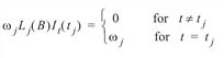
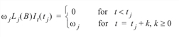
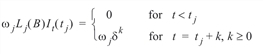
Assuming the outlier occurs at time point tj, the outlier impact is shown in Outlier Impact:
|
Outlier |
Formula |
|---|---|
|
Innovational outliers (IO) |
|
|
Additive outliers (AO) |
|
|
Level shifts (LS) |
|
|
Temporary changes (TC) |
|
From these formulas, the forecasts  can be computed easily.
The 100(1 – a) percent probability limits for  and Yt+1 are given by:
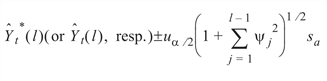
where  is the 100(1 – a/2) percentile of the standard normal distribution,
  is an estimate of the variance
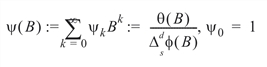
  of the random shocks (returned from TS_OUTLIER_IDENTIFICATION), and the y weights {yj} are the coefficients in:
Example
This example is a realization of an ARMA(2,1) process described by the model Yt – Yt–1 + 0.24Yt–2 = 10.0 + at + 0.5at–1, {at} a Gaussian white noise process. Outliers were artificially added to the outlier free series {Yt}t=1, ..., 280 at time points t = 150 (level shift, w1 = +2.5) and t = 200 (additive outlier, w2 = +3.2), resulting in the outlier contaminated series {Zt}t=1, ..., 280. For both series, forecasts were determined for time points t = 281, ..., 290 and compared with the actual values of the series.
time_series = [ $
41.67 , 41.67 , 42.0752144, 42.6123962, $
43.6161919, 42.1932831, 43.1055450, 44.3518715, $
45.3961258, 45.0790215, 41.8874397, 40.2159805, $
40.2447319, 39.6208458, 38.6873589, 37.9272423, $
36.8718872, 36.8310852, 37.4524879, 37.3440933, $
37.9861374, 40.3810501, 41.3464622, 42.6495285, $
42.6096764, 40.3134537, 39.7971268, 41.5401535, $
40.7160759, 41.0363541, 41.8171883, 42.4190292, $
43.0318832, 43.9968109, 44.0419617, 44.3225212, $
44.6082611, 43.2199631, 42.0419197, 41.9679718, $
42.4926224, 43.2091255, 43.2512283, 41.2301674, $
40.1057358, 40.4510574, 41.5329170, 41.5678177, $
43.0090141, 42.1592140, 39.9234505, 38.8394127, $
40.4319878, 40.8679352, 41.4551926, 41.9756317, $
43.9878922, 46.5736389, 45.5939293, 42.4487762, $
41.5325394, 42.8830910, 44.5771217, 45.8541985, $
46.8249474, 47.5686378, 46.6700745, 45.4120026, $
43.2305107, 42.7635345, 43.7112923, 42.0768661, $
41.1835632, 40.3352280, 37.9761467, 35.9550056, $
36.3212509, 36.9925880, 37.2625008, 37.0040665, $
38.5232544, 39.4119797, 41.8316803, 43.7091446, $
42.9381447, 42.1066780, 40.3771248, 38.6518707, $
37.0550499, 36.9447708, 38.1017685, 39.4727097, $
39.8670387, 39.3820763, 38.2180786, 37.7543488, $
37.7265244, 38.0290642, 37.5531158, 37.4685936, $
39.8233147, 42.0480766, 42.4053535, 43.0117416, $
44.1289330, 45.0393829, 45.1114540, 45.0086479, $
44.6560631, 45.0278931, 46.7830849, 48.7649765, $
47.7991905, 46.5339661, 43.3679199, 41.6420822, $
41.2694893, 41.5959740, 43.5330009, 43.3643608, $
42.1471291, 42.5552788, 42.4521446, 41.7629128, $
39.9476891, 38.3217010, 40.5318718, 42.8811569, $
44.4796944, 44.6887932, 43.1670265, 41.2226143, $
41.8330154, 44.3721924, 45.2697029, 44.4174194, $
43.5068550, 44.9793015, 45.0585403, 43.2746620, $
40.3317070, 40.3880501, 40.2627106, 39.6230278, $
41.0305252, 40.9262009, 40.8326912, 41.7084885, $
42.9038048, 45.8650513, 46.5231590, 47.9916115, $
47.8463135, 46.5921936, 45.8854408, 45.9130440, $
45.7450371, 46.2964249, 44.9394569, 45.8141251, $
47.5284042, 48.5527802, 48.3950577, 47.8753052, $
45.8880005, 45.7086983, 44.6174774, 43.5567932, $
44.5891113, 43.1778679, 40.9405632, 40.6206894, $
41.3330421, 42.2759552, 42.4744949, 43.0719833, $
44.2178459, 43.8956337, 44.1033440, 45.6241455, $
45.3724861, 44.9167595, 45.9180603, 46.9077835, $
46.1666603, 46.6013489, 46.6592331, 46.7291603, $
47.1908340, 45.9784355, 45.1215782, 45.6791115, $
46.7379875, 47.3036957, 45.9968834, 44.4669495, $
45.7734680, 44.6315041, 42.9911766, 46.3842583, $
43.7214432, 43.5276833, 41.3946495, 39.7013168, $
39.1033401, 38.5292892, 41.0096245, 43.4535828, $
44.6525154, 45.5725899, 46.2815285, 45.2766647, $
45.3481712, 45.5039482, 45.6745682, 44.0144806, $
42.9305000, 43.6785469, 42.2500534, 40.0007210, $
40.4477005, 41.4432716, 42.0058670, 42.9357758, $
45.6758842, 46.8809929, 46.8601494, 47.0449791, $
46.5420647, 46.8939934, 46.2963371, 43.5479164, $
41.3864059, 41.4046364, 42.3037987, 43.6223717, $
45.8602371, 47.3016396, 46.8632469, 45.4651413, $
45.6275482, 44.9968376, 42.7558670, 42.0218239, $
41.9883728, 42.2571678, 44.3708687, 45.7483635, $
44.8832512, 44.7945862, 44.8922577, 44.7409401, $
45.1726494, 45.5686874, 45.9946709, 47.3151054, $
48.0654068, 46.4817467, 42.8618279, 42.4550323, $
42.5791168, 43.4230957, 44.7787971, 43.8317108, $
43.6481781, 42.4183960, 41.8426285, 43.3475227, $
44.4749908, 46.3498306, 47.8599319, 46.2449913, $
43.6044006, 42.4563484, 41.2715340, 39.8492508, $
39.9997292, 41.4410820, 42.9388237, 42.5687332]
; We will use the first 280 to generate a forecast for the
; next 10 and test that forecast against these 10 actual
; observations.
forecast_actual = [42.6384087, 41.7088661, 43.9399033, $
45.4284401, 44.4558411, 45.1761856, $
45.3489113, 45.1892662, 46.3754730, $
45.6082802]
delta = 0.7
n_predict = 10
model = [2, 1, 1, 0]
result = TS_OUTLIER_IDENTIFICATION( $
model, time_series, $
Relative_Error=1.0e-4, $
Num_Outliers=num_outliers, $
Residual=residual, $
Outlier_Statistics=outlier_stat, $
Omega_Weights=omega, $
Arma_Param=parameters, $
Res_Sigma=res_sigma, $
Aic=aic)
PRINT, "ARMA parameters:"
PRINT, parameters, Format='(F11.6)'
PRINT, ''
PRINT, num_outliers, Format="('Number of outliers: ', I1)"PRINT, ''
PRINT, "Outlier statistics:"
PRINT, "Time point Outlier type"
FOR i=0L, num_outliers-1 DO $
PRINT, outlier_stat(i,0), outlier_stat(i,1), $
Format="(I6, 10X, I3)"
PRINT, ''
PRINT, res_sigma, Format="('RSE: ', F11.6)"PRINT, aic, Format="('AIC: ', F11.6)"PRINT, ''
; collect the output from the TS_OUTLIER_IDENTIFICATION call
; and arrange it for the call to TS_OUTLIER_FORECAST
series = FLTARR(N_ELEMENTS(time_series),2)
series(*,0) = time_series
series(*,1) = residual
forecast = TS_OUTLIER_FORECAST( $
series, $
outlier_stat, omega, delta, $
model, parameters, n_predict, $
Out_Free_Forecast=outfree_forecast)
forecast_table = FLTARR(n_predict,4)
PRINT, "** " + $
"Forecast Table for Outlier Contaminated Series **"
PRINT, "Orig. Series Forecast Prob. Limits PSI Weights"
FOR i=0L, n_predict-1 DO $
PRINT, forecast_actual(i), forecast(i,0), $
forecast(i,1), forecast(i,2), $
Format='(F10.4, 3F13.4)'
PRINT, ''
PRINT, "****** " + $
"Forecast Table for Outlier Free Series ******"
PRINT, " Outlier"
PRINT, " Free Series Forecast Prob. Limits PSI Weights"
FOR i=0L, n_predict-1 DO BEGIN & $
PRINT, forecast_actual(i), outfree_forecast(i,0), $
outfree_forecast(i,1), outfree_forecast(i,2), $
Format='(F10.4, 3F13.4)' & $
ENDFOR
Output
ARMA parameters:
8.891920
0.944060
-0.150423
-0.558918
Number of outliers: 2
Outlier statistics:
Time point Outlier type
150 2
200 1
RSE: 1.004306
AIC: 1323.617554
** Forecast Table for Outlier Contaminated Series **
Orig. Series Forecast Prob. Limits PSI Weights
42.6384 43.6852 1.9684 1.5030
41.7089 43.8266 3.5535 1.2685
43.9399 44.0516 4.3430 0.9714
45.4284 44.2428 4.7453 0.7263
44.4558 44.3895 4.9560 0.5395
45.1762 44.4992 5.0685 0.4001
45.3489 44.5807 5.1293 0.2966
45.1893 44.6411 5.1624 0.2198
46.3755 44.6859 5.1805 0.1629
45.6083 44.7191 5.1904 0.1207
****** Forecast Table for Outlier Free Series ******
Outlier
Free Series Forecast Prob. Limits PSI Weights
40.1384 41.9598 1.9684 1.5030
39.2089 42.1012 3.5535 1.2685
41.4399 42.3262 4.3430 0.9714
42.9284 42.5174 4.7453 0.7263
41.9558 42.6641 4.9560 0.5395
42.6762 42.7738 5.0685 0.4001
42.8489 42.8553 5.1293 0.2966
42.6893 42.9157 5.1624 0.2198
43.8755 42.9605 5.1805 0.1629
43.1083 42.9937 5.1904 0.1207


