STRIP_SPLIT_PLOT Function
Analyzes data from strip-split-plot experiments. STRIP_SPLIT_PLOT also analyzes strip-split-plot experiments replicated at several locations.
Usage
result = STRIP_SPLIT_PLOT (n, n_locations, n_strip_a, n_strip_b, n_split, block, strip_a, strip_b, split, y)
Input Parameters
n—Number of missing and non-missing experimental observations. STRIP_PLOT verifies that:
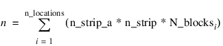
where N_blocksi is equal to the number of blocks or replicates at the ith location.
n_locations—Number of locations. n_locations must be one or greater. If n_locations > 1 then the Locations keywords must be included as input to STRIP_SPLIT_PLOT.
n_strip_a—Number of levels associated with the strip-plot A factor. n_strip_a must be greater than one.
n_strip_b—Number of levels associated with the strip-plots B factor. n_strip_b must be greater than one.
n_split—Number of levels associated with the split factor. n_split must be greater than one.
block—Array of length n containing the block identifiers for each observation in y. Locations can have different numbers of blocks. Each block at a single location must be assigned a different identifier, but different locations can have the same assignments.
strip_a—Array of length n containing the strip-plot A level identifiers for each observation in y. Each level of this factor must be assigned a different integer. STRIP_SPLIT_PLOT verifies that the number of unique strip-plot identifiers is equal to n_strip_a.
strip_b—Array of length n containing the strip-plot B identifiers for each observation in y. Each level of this factor must be assigned a different integer. STRIP_SPLIT_PLOT verifies that the number of unique strip-plot identifiers is equal to n_strip_b.
split—Array of length n containing the split-plot level identifiers for each observation in y. Each level of this factor must be assigned a different integer. STRIP_SPLIT_PLOT verifies that the number of unique split-plot identifiers is equal to n_split.
y—Array of length n containing the experimental observations and any missing values. Missing values cannot be omitted. They are indicated by placing a NaN (Not a Number) at the appropriate positions in y. NaN can be defined by calling the MACHINE function. For example:
x = MACHINE(/Float)
y(i) = x.NaN
The location, strip-plot A, strip-plot B and split-plot for each observation in y are identified by the corresponding values in the Locations keyword, and the input parameters strip_a, strip_b, and split.
Returned Value
result—A two dimensional, 22 by 6 array containing the ANOVA table. Each row in this array contains values for one of the effects in the ANOVA table. The first value in each row, anova_tablei,0 = anova_table(i,0), identifies the source for the effect associated with values in that row. The remaining values in a row contain the ANOVA table values using the convention found in ANOVA Table Values.
|
J |
anova_tablei,j = anova_table(i,j) |
|---|---|
|
0 |
Source Identifier (values described below) |
|
1 |
Degrees of freedom |
|
2 |
Sum of squares |
|
3 |
Mean squares |
|
4 |
F-statistic |
|
5 |
p-value for this F-statistic |
The Source Identifiers in the first column of anova_tablei,j are the only negative values in anova_table. Assignments of identifiers to ANOVA sources use the coding shown in ANOVA Assignment Identifiers.
|
Source Identifier |
ANOVA Source |
|---|---|
|
-1 |
LOCATIONS* |
|
-2 |
BLOCK WITHIN LOCATION |
|
-3 |
STRIP-PLOT A |
|
-4 |
LOCATION × STRIP-PLOT A* |
|
-5 |
STRIP-PLOT A ERROR |
|
-6 |
SPLIT-PLOT |
|
-7 |
SPLIT-PLOT × STRIP-PLOT A |
|
-8 |
LOCATION × SPLIT-PLOT* |
|
-9 |
SPLIT-PLOT ERROR |
|
-10 |
LOCATION × SPLIT-PLOT × STRIP-PLOT A* |
|
-11 |
STRIP-PLOT B |
|
-12 |
LOCATION × STRIP-PLOT B* |
|
-13 |
STRIP_PLOT B ERROR |
|
-14 |
STRIP-PLOT A × STRIP-PLOT B |
|
-15 |
LOCATION × STRIP-PLOT A × STRIP-PLOT B |
|
-16 |
STRIP-PLOT A × STRIP-PLOT B ERROR |
|
-17 |
SPLIT-PLOT × STRIP-PLOT B |
|
-18 |
STRIP-PLOT A × STRIP-PLOT B × SPLIT-PLOT |
|
-19 |
LOCATION × SPLIT-PLOT × STRIP-PLOT B* |
|
-20 |
LOCATION × STRIP-PLOT A × STRIP-PLOT B × SPLIT-PLOT* |
|
-21 |
STRIP-PLOT A × STRIP-PLOT B × SPLIT-PLOT ERROR |
|
-22 |
CORRECTED TOTAL |
|
* If n_locations = 1 sources involving location are set to missing (NaN). |
|
Input Keywords
Double—If present and nonzero, double precision is used.
Locations—Array of length n containing the location identifiers for each observation in y. Unique integers must be assigned to each location in the study. This keyword is required when n_locations > 1.
Output Keywords
N_missing—Number of missing values, if any, found in y. Missing values are denoted with a NaN (Not a Number) value.
Cv—Array of length 3 containing the strip-plots and split-plot coefficients of variation. Cv(0) contains the strip-plot A C.V., Cv(1) contains the strip-plot B C.V., and Cv(2) contains the split-plot C.V.
Grand_mean—Mean of all the data across every location.
Strip_plot_a_means—Array of length n_strip_a containing the factor A strip-plot means.
Strip_plot_b_means—Array of length n_strip_b containing the strip-plot B means.
Split_plot_means—Array of length n_split containing the strip-plot B means.
Strip_plot_a_split_plot_means—A 2-dimensional array of size n_strip_a by n_split containing the means for all combinations of the factor A strip-plot and split-plots.
Split_plot_b_split_plot_means—A 2-dimensional array of size n_strip_b by n_split containing the means for all combinations of strip-plot B and split-plots.
Strip_plot_ab_means—A 2-dimensional array of size n_strip_a by n_strip_b containing the means for all combinations of strip-plots.
Treatment_means—Array of size (n_strip_a by n_strip_b by n_split) containing the treatment means. For i > 0 and j > 0, Treatment_meansi,j contains the mean of the observations, averaged over all locations, blocks and replicates, for the ith level of the strip-plot and the jth level of the split-plot.
Std_errors—Array of length 20 containing ten standard errors and their associated degrees of freedom. The standard errors are in the first 10 elements and their associated degrees of freedom are reported in Std_errors(10) through Std_errors(19). Refer to Standard Errors for a list of the standard errors and their associated degrees of freedom.
|
Element |
Standard Error for Comparisons Between Two |
Degrees of Freedom |
|---|---|---|
|
Std_errors(0) |
Strip-Plot A Means |
Std_errors(10) |
|
Std_errors(1) |
Strip-Plot B Means |
Std_errors(11) |
|
Std_errors(2) |
Split-Plot Means |
Std_errors(12) |
|
Std_errors(3) |
Strip-Plot A Means at the same level of split-plots |
Std_errors(13) |
|
Std_errors(4) |
Strip-Plot A Means at the same level of strip-plot B |
Std_errors(14) |
|
Std_errors(5) |
Strip-Plot B Means at the same level of split-plots |
Std_errors(15) |
|
Std_errors(6) |
Strip-Plot B Means at the same level of strip-plot A |
Std_errors(16) |
|
Std_errors(7) |
Split-Plot Means at the same level of split-plot A |
Std_errors(17) |
|
Std_errors(8) |
Split-Plot Means at the same level of strip-plot B |
Std_errors(18) |
|
Std_errors(9) |
Treatment Means (same strip-plot A, strip-plot B and split-plot) |
Std_errors(19) |
N_blocks—Array of length n_locations containing the number of blocks, or replicates, at each location. This value must be greater than one.
Location_anova_table—A 3-dimensional array of size n_locations by 22 by 6 containing the ANOVA tables associated with each location. For each location, the 22 by 6 dimensional array corresponds to the ANOVA table for that location. For example, Location_anova_table(i,j,k) contains the value in the kth column and jth row of the returned anova-table for the ith location.
Anova_row_labels—Array containing the labels for each of the rows of the returned ANOVA table. The label for the ith row of the ANOVA table can be printed with PRINT, Anova_row_labels(i).
Discussion
STRIP_SPLIT_PLOT is capable of analyzing a wide variety of strip-split plot experiments, also referred to as strip-strip plot experiments. By default, STRIP_SPLIT_PLOT assumes that both strip-plot factors, and split-plots are fixed effects, and the location effects, if any, are random effects. The nature of randomization used in an experiment determines analysis of the data. Two popular forms of randomization in strip-plot and split-plot experiments are illustrated in Strip-Plot Experiment—Strip-Plots Completely Crossed and Split-Plot Experiment—Factor B Split-Plots Nested within Factor A Whole-Plots. In both experiments, the strip-plot factor, factor A, has 4 levels that are randomly assigned to a block or field in four strips.
|
|
|
Factor A Strip-Plots |
|||
|
|
|
A2 |
A1 |
A4 |
A3 |
|
Factor B Strip Plots |
B3 |
A2B3 |
A1B3 |
A4B3 |
A3B3 |
|
B1 |
A2B1 |
A1B1 |
A4B1 |
A3B1 |
|
|
B2 |
A2B2 |
A1B2 |
A4B2 |
A3B2 |
|
In the strip-plot experiment, factor B, has 3 levels that are randomly assigned as strips across each of the four levels of factor A. In this case, factors A and B are completely crossed. The randomization applied to factor B is independent of the application of the strip-plots, factor A.
Contrast this to the randomization depicted in Split-Plot Experiment—Factor B Split-Plots Nested within Factor A Whole-Plots. In this split-plot experiment, the levels of factor B are nested within each level of factor A whole-plots. Factor B is randomized independently within each level of factor A. Unlike the strip-plot experiment, in the split-plot experiment different levels of factor B appear in the same row.
|
Whole-Plot Factor |
|||
|---|---|---|---|
|
A2 |
A1 |
A4 |
A3 |
|
A2B1 |
A1B3 |
A4B1 |
A3B3 |
|
A2B3 |
A1B1 |
A4B3 |
A3B1 |
|
A2B2 |
A1B2 |
A4B2 |
A3B2 |
A strip-split plot experiment is a strip-plot experiment with a third factor randomized within each level of strip-plot factor A, see Strip-Split Plot Experiment—Split-Plots nested within Strip-Plot Factors A. The third factor, referred to as the split-plot factor, is randomly assigned to experimental units within each level of strip-plot factor A. STRIP_SPLIT_PLOT analyzes strip-split plot experiments consisting of two strip-plot factors and one split-plot factor nested within strip-plot factors A and B.
Strip-split plot experiments are closely related to split-split plot experiments, see Sub-Plot Factor C Nested Within Split-Plot Factor B, Nested Within Whole-Plot Factor A. The main difference between the two is that in strip-split plot experiments, the order of the levels for factor B are not applied randomly across factor A. Each level of factor B is constant across any row. In this example, the entire first row is assigned to the third level of factor B. In the equivalent split-split plot experiment, the levels of factor B are not constant across any row. The levels are randomized within each level of factor A.
In some studies, a strip-split-plot experiment is replicated at several locations. STRIP_SPLIT_PLOT can analyze strip-split plot experiments replicated at multiple locations, even when the number of blocks or replicates at each location might be different different. If only a single replicate or block is used at each location, then location should be treated as a blocking factor, with n_locations = 1. If n_locations = 1, it is assumed that either the experiment was conducted at multiple locations, each with a single block, or at a single location with more than one block or replicate at that location. When n_locations = 1, all entries associated with location in the ANOVA table will contain missing values.
However, if n_locations > 1, it is assumed the experiment was repeated at multiple locations, with blocking occurring at each location. Although the number of blocks at each location can be different, the number of levels for the strip-plot and split-plot factors strip-plots must be the same at each location. The locations associated with each of the observations in y are specified by the Locations keyword, which is a required keyword when n_locations > 1.
By default, locations are assumed to be random effects. Tests involving strip-plots use the interaction between strip-plots and locations as the error term for testing whether there are statistically significant differences among strip-plots. However, this assumes that the interaction of strip-plots and locations is not statistically significant. A test of this assumption is included in the ANOVA table. If any interactions between locations and strip-plot or split-plot factors are statistically significant, then the nature of these interactions should be explored since this impacts the interpretation of the significance of the treatment factors.
Similarly, when locations are assumed to be random effects, tests involving split-plots do not use the split-plot errors pooled across locations. Instead, the error term for split-plots is the interaction between locations and split-plots.
Suppose, for example, that a researcher wanted to conduct an agricultural experiment comparing the effectiveness of 4 fertilizers with 3 seed lots and 3 rates of application. One replicate of the experiment is conducted at each of the 3 farms. That is, only a single field at each location is assigned to this experiment.
Each field is divided into 4 vertical strips and 3 horizontal strips. The vertical strips are randomly assigned to fertilizers and the rows are randomly assigned to application rates. Fertilizers and application rates represent strip-plot factors A and B respectively. Seed lots are randomly assigned to three sub-divisions within each combination of strip-plots.
|
|
|
Fertilizer Strip Plots |
|||
|
|
|
F2 |
F1 |
F4 |
F3 |
|
Application Rate Strip Plot |
R3 |
F2R3S1 |
F1R3S3 |
F4R3S3 |
F3R3S2 |
|
R2 |
F2R1S3 |
F1R1S2 |
F4R1S3 |
F3R1S1 |
|
|
R1 |
F2R2S1 |
F1R2S1 |
F4R2S2 |
F3R2S3 |
|
In this case, each farm is a blocking factor, fertilizers are factor A strip-plots, fertilizer application rates are factor B strip-plots, and seed lots are split-plots. The input array for the Locations keyword would contain integers from 1 to the number of farms.
Example
The experiment was conducted using a 2x2 strip_split plot arrangement with each of the four plots divided into 2 sub-divisions that were randomly assigned one of two split-plot levels. This was replicated 3 times producing an experiment with n = 2x2x2x3 = 24 observations.
; Total number of observations
n = 24
; Number of locations
n_locations = 1
; Number of factor A strip-plots within a location
n_strip_a = 2
; Number of factor B strip-plots within a location
n_strip_b = 2
; Number of split-plots within each Factor A strip-plot
n_split = 2
block = [1, 1, 1, 1, 1, 1, 1, 1, $
2, 2, 2, 2, 2, 2, 2, 2, $
3, 3, 3, 3, 3, 3, 3, 3]
strip_a = [1, 1, 1, 1, 2, 2, 2, 2, $
1, 1, 1, 1, 2, 2, 2, 2, $
1, 1, 1, 1, 2, 2, 2, 2]
strip_b = [1, 1, 2, 2, 1, 1, 2, 2, $
1, 1, 2, 2, 1, 1, 2, 2, $
1, 1, 2, 2, 1, 1, 2, 2]
split = [1, 2, 1, 2, 1, 2, 1, 2, $
1, 2, 1, 2, 1, 2, 1, 2, $
1, 2, 1, 2, 1, 2, 1, 2]
y = [30.0, 40.0, 38.9, 38.2, $
41.8, 52.2, 54.8, 58.2, $
20.5, 26.9, 21.4, 25.1, $
26.4, 36.7, 28.9, 35.9, $
21.0, 25.4, 24.0, 23.3, $
34.4, 41.0, 33.0, 34.9]
aov = STRIP_SPLIT_PLOT(n, n_locations, n_strip_a, $
n_strip_b, n_split, block, $
strip_a, strip_b, split, y, $
Cv=cv, Grand_mean=grand_mean, $
Treatment_means=treatment_means, $
Strip_plot_a_means= $
strip_plot_a_means, $
Strip_plot_b_means=$
strip_plot_b_means, $
Split_plot_means=split_plot_means, $
Strip_plot_a_split_plot_means= $
strip_plot_a_split_plot_means, $
Strip_plot_b_split_plot_means= $
strip_plot_b_split_plot_means, $
Strip_plot_ab_means= $
strip_plot_ab_means, $
Std_errors=std_errors, $
N_blocks=n_blocks, $
Location_anova_table= $
location_anova_table)
labels = ['Location ', $
'Blocks ', $
'Strip-Plot A ', $
'Location x A ', $
'Strip-Plot A Error ', $
'Split-Plot ', $
'Split-Plot x A ', $
'Location x ', $
' Split-Plot ', $
'Split-Plot Error ', $
'Location x ', $
' Split-Plot x A ', $
'Strip-Plot B ', $
'Location x B ', $
'Strip-Plot B Error ', $
'A x B ', $
'Location x A x B ', $
'A x B Error ', $
'Split-Plot x B ', $
'Split-Plot x A x B ', $
'Location x ', $
' Split-Plot x B ', $
'Location x ', $
' Split-Plot x A x B', $
'Split-Plot x A x ', $
' B Error ', $
'Corrected Total ']
; Print Analysis of Variance Table
PRINT, " *** ANALYSIS OF VARIANCE TABLE ***"
PRINT, 'ID', 'DF', 'SSQ', 'MS', 'F-Test', 'p-Value', $
Format='(A24, A5, A9, A8, A7, A8)'
idx = 0
FOR i=0L, (SIZE(aov))(1)-1 DO BEGIN & $
PRINT, labels(idx), aov(i,0), aov(i,1), aov(i,2), $
aov(i,3), aov(i,4), aov(i,5), Format= $
'(A20, 1X, I3, 2X, F3.0, 2X, F7.2, 2X, F6.2, 2X, ' + $
'F5.2, 2X, F6.3)' & $
idx = idx + 1 & $
IF idx LT N_ELEMENTS(labels)-1 THEN $
WHILE STRPOS(labels(idx), ' ', 0) EQ 0 DO BEGIN & $
PRINT, labels(idx) & idx = idx + 1 & $
ENDWHILE & $
ENDFOR
PRINT, ''
PRINT, grand_mean, Format="('Grand mean: ', F9.6, '\012')"PRINT, "Coefficient of Variation"
labels = ['Strip-Plot A:', 'Strip-Plot B:','Strip-Plot: ']
FOR i=0L, 2 DO PRINT, labels(i), cv(i), Format='(A15, F12.4)'
PRINT, ''
PRINT, "****************************************************"
; Print the Treatment Means
PRINT, "Treatment Means"
idx = 0
FOR i=0L, n_strip_a-1, idx+1 DO $
FOR j=0L, n_strip_b-1 DO $
FOR k=0L, n_split-1 DO $
PRINT, (i+1), (j+1), (k+1), $
treatment_means(i,j,k), Format= "('" + $" Treatment[', I1, '][', I1, '][', I1, '] Mean:', F9.4)"
PRINT, ''
PRINT, std_errors(9), $
Format='("Standard Error for Comparing Two ' + $'Treatment Means:", F9.6)'
PRINT, std_errors(19), Format="('(df=', F8.6, ')', '\012')"; Perform multiple comparison using the LSD procedure
equal_means = MULTICOMP(REFORM(treatment_means, $
(n_strip_a*n_strip_b*n_split)), $
std_errors(19), std_errors(9)/SQRT(2.0), $
/LSD, Alpha=0.05)
PM, equal_means, $
Title="LSD Comparison: Size of Groups of Means"
PRINT, ''
PRINT, "****************************************************"
; Print the Strip-plot A Means.
;
PM, strip_plot_a_means, Title="Strip-plot A means"
PRINT, ''
PRINT, std_errors(0), $
Format='("Standard Error for Comparing Two ' + $'Strip-Plot A Means:", F9.6)'
PRINT, std_errors(10), Format="('(df=', F8.6, ')', '\012')"; Perform multiple comparison using the LSD procedure
equal_means = MULTICOMP(strip_plot_a_means, $
std_errors(10), std_errors(0)/SQRT(2.0), $
/LSD, Alpha=0.05)
PM, equal_means, $
Title="LSD Comparison: Size of Groups of Means"
PRINT, ''
PRINT, "****************************************************"
; Print the Strip-plot B Means.
;
PM, strip_plot_b_means, Title="Strip-plot B means"
PRINT, ''
PRINT, std_errors(1), $
Format='("Standard Error for Comparing Two ' + $'Strip-Plot B Means:", F9.6)'
PRINT, std_errors(11), Format="('(df=', F8.6, ')', '\012')"; Perform multiple comparison using the LSD procedure
equal_means = MULTICOMP(strip_plot_b_means, $
std_errors(11), std_errors(1)/SQRT(2.0), $
/LSD, Alpha=0.05)
PM, equal_means, $
Title="LSD Comparison: Size of Groups of Means"
PRINT, ''
PRINT, "****************************************************"
; Print the Split-plot Means.
PM, split_plot_means, Title="Split-plot Means"
PRINT, ''
PRINT, std_errors(2), $
Format='("Standard Error for Comparing Two ' + $'Split-Plot Means:", F9.6)'
PRINT, std_errors(12), Format="('(df=', F8.6, ')', '\012')"; Perform multiple comparison using the LSD procedure
equal_means = MULTICOMP(split_plot_means, $
std_errors(12), std_errors(2)/SQRT(2.0), $
/LSD, Alpha=0.05)
PM, equal_means, $
Title="LSD Comparison: Size of Groups of Means"
PRINT, ''
PRINT, "****************************************************"
; Print the Strip-plot A by Split-plot Means.
PM, strip_plot_a_split_plot_means, $
Title="Strip-plot A by Split-plot Means"
PRINT, ''
PRINT, std_errors(3), $
Format='("Standard Error for Comparing Two Means:", F9.6)'PRINT, std_errors(13), Format="('(df=', F8.6, ')', '\012')"; Perform multiple comparison using the LSD procedure
equal_means = MULTICOMP( $
REFORM(strip_plot_a_split_plot_means, $
n_strip_a*n_split), $
std_errors(13), std_errors(3)/SQRT(2.0), $
/LSD, Alpha=0.05)
PM, equal_means, $
Title="LSD Comparison: Size of Groups of Means"
PRINT, ''
PRINT, "****************************************************"
; Print the Strip-plot A by Split-plot B Means.
;
PM, strip_plot_ab_means, $
Title="Strip-plot A by Strip-plot B Means"
PRINT, ''
PRINT, std_errors(4), $
Format='("Standard Error for Comparing Two Means:", F9.6)'PRINT, std_errors(14), Format="('(df=', F8.6, ')', '\012')"; Perform multiple comparison using the LSD procedure
equal_means = MULTICOMP(REFORM(strip_plot_ab_means, $
n_strip_a*n_strip_b), $
std_errors(14), std_errors(4)/SQRT(2.0), $
/LSD, Alpha=0.05)
PM, equal_means, $
Title="LSD Comparison: Size of Groups of Means"
PRINT, ''
PRINT, "****************************************************"
; Print the Strip-plot B by Split-plot Means.
PM, strip_plot_b_split_plot_means, $
Title="Strip-plot B by Split-plot Means"
PRINT, ''
PRINT, std_errors(5), $
Format='("Standard Error for Comparing Two Means:", F9.6)'PRINT, std_errors(15), Format="('(df=', F8.6, ')', '\012')"PRINT, ''
; Perform multiple comparison using the LSD procedure
equal_means = MULTICOMP($
REFORM(strip_plot_b_split_plot_means, $
n_strip_b*n_split), $
std_errors(15), std_errors(5)/SQRT(2.0), $
/LSD, Alpha=0.05)
PM, equal_means, $
Title="LSD Comparison: Size of Groups of Means"
PRINT, ''
Output
*** ANALYSIS OF VARIANCE TABLE ***
ID DF SSQ MS F-Test p-Value
Location -1 NaN NaN NaN NaN NaN
Blocks -2 2. 1310.28 655.14 14.53 0.061
Strip-Plot A -3 1. 858.01 858.01 40.37 0.024
Location x A -4 NaN NaN NaN NaN NaN
Strip-Plot A Error -5 2. 42.51 21.26 1.48 0.385
Split-Plot -6 1. 163.80 163.80 41.22 0.003
Split-Plot x A -7 1. 11.34 11.34 2.85 0.166
Location x -8 NaN NaN NaN NaN NaN
Split-Plot
Split-Plot Error -9 4. 15.90 3.97 1.56 0.338
Location x -10 NaN NaN NaN NaN NaN
Split-Plot x A
Strip-Plot B -11 1. 17.17 17.17 0.47 0.565
Location x B -12 NaN NaN NaN NaN NaN
Strip-Plot B Error -13 2. 73.51 36.75 2.85 0.260
A x B -14 1. 1.55 1.55 0.12 0.762
Location x A x B -15 NaN NaN NaN NaN NaN
A x B Error -16 2. 25.82 12.91 5.08 0.080
Split-Plot x B -17 1. 46.76 46.76 18.39 0.013
Split-Plot x A x B -18 1. 0.51 0.51 0.20 0.677
Location x -19 NaN NaN NaN NaN NaN
Split-Plot x B
Location x -20 NaN NaN NaN NaN NaN
Split-Plot x A x B
Split-Plot x A x -21 4. 10.17 2.54 NaN NaN
B Error
Corrected Total -22 23. 2577.33 NaN NaN NaN
Grand mean: 33.870834
Coefficient of Variation
Strip-Plot A: 13.6116
Strip-Plot B: 17.8986
Strip-Plot: 5.8854
****************************************************
Treatment Means
Treatment[1][1][1] Mean: 23.8333
Treatment[1][1][2] Mean: 30.7667
Treatment[1][2][1] Mean: 28.1000
Treatment[1][2][2] Mean: 28.8667
Treatment[2][1][1] Mean: 34.2000
Treatment[2][1][2] Mean: 43.3000
Treatment[2][2][1] Mean: 38.9000
Treatment[2][2][2] Mean: 43.0000
Standard Error for Comparing Two Treatment Means: 1.302029
(df=4.000000)
LSD Comparison: Size of Groups of Means
0
3
0
2
0
0
2
****************************************************
Strip-plot A means
27.8917
39.8500
Standard Error for Comparing Two Strip-Plot A Means: 1.882171
(df=2.000000)
LSD Comparison: Size of Groups of Means
0
****************************************************
Strip-plot B means
33.0250
34.7167
Standard Error for Comparing Two Strip-Plot B Means: 2.474972
(df=2.000000)
LSD Comparison: Size of Groups of Means
2
****************************************************
Split-plot Means
31.2583
36.4833
Standard Error for Comparing Two Split-Plot Means: 0.813813
(df=4.000000)
LSD Comparison: Size of Groups of Means
0
****************************************************
Strip-plot A by Split-plot Means
25.9667 29.8167
36.5500 43.1500
Standard Error for Comparing Two Means: 1.150906
(df=4.000000)
LSD Comparison: Size of Groups of Means
0
0
0
****************************************************
Strip-plot A by Strip-plot B Means
27.3000 28.4833
38.7500 40.9500
Standard Error for Comparing Two Means: 2.074280
(df=2.000000)
LSD Comparison: Size of Groups of Means
2
0
2
****************************************************
Strip-plot B by Split-plot Means
29.0167 37.0333
33.5000 35.9333
Standard Error for Comparing Two Means: 0.920673
(df=4.000000)
LSD Comparison: Size of Groups of Means
0
2
2


