LATIN_SQUARE Function
Analyzes data from latin-square experiments. LATIN_SQUARE also analyzes latin-square experiments replicated at several locations.
Usage
result = latin_square (n, n_locations, n_treatments, row, col, treatment, y)
Input Parameters
n—Number of missing and non-missing experimental observations. LATIN_SQUARE verifies that:
n_locations—Number of locations. Must be greater than or equal to one. If n_locations > 1 then the Locations keyword must be included as input to LATIN_SQUARE.
n_treatments—Number of treatments. n_treatments must be greater than one. In addition, the number of unique row and column identifiers specified in the input parameters row and col must be equal to n_treatments.
row—Array of length n containing the row identifiers for each observation in y. Each row must be assigned values from 1 to n_treatments. LATIN_SQUARE verifies that the number of unique factor A identifiers is equal to n_treatments.
col—Array of length n containing the column identifiers for each observation in y. Each column must be assigned values from 1 to n_treatments. LATIN_SQUARE verifies that the number of unique column identifiers is equal to n_treatments.
treatment—Array of length n containing the treatment identifiers for each observation in y. Each treatment must be assigned values from 1 to n_treatments. LATIN_SQUARE verifies that the number of unique treatment identifiers is equal to n_treatments.
y—Array of length n containing the experimental observations and any missing values. Missing values cannot be omitted. They are indicated by placing a NaN (Not a Number) at the appropriate positions in y. NaN can be defined by calling the MACHINE function. For example:
x = MACHINE(/Float)
y(i) = x.NaN
The location, row, column, and treatment number for each observation in y are identified by the corresponding values in Locations, row, col, and n_treatments.
Returned Value
result—A two dimensional, 7 by 6 array containing the ANOVA table. Each row in this array contains values for one of the effects in the ANOVA table. The first value in each row, anova_tablei,0 = anova_table(i,0), identifies the source for the effect associated with values in that row. The remaining values in a row contain the ANOVA table values shown in ANOVA Table Values.
|
J |
anova_tablei,j = anova_table(i,j) |
|---|---|
|
0 |
Source Identifier (values described below) |
|
1 |
Degrees of freedom |
|
2 |
Sum of squares |
|
3 |
Mean squares |
|
4 |
F-statistic |
|
5 |
p-value for this F-statistic |
The Source Identifiers in the first column of anova_tablei,j are the only negative values in anova_table. Assignments of identifiers to ANOVA sources use the coding shown in ANOVA Assignment Identifiers:
|
Source Identifier |
ANOVA Source |
|---|---|
|
–1 |
LOCATIONS* |
|
–2 |
ROWS |
|
–3 |
COLUMNS |
|
–4 |
TREATMENTS |
|
–5 |
LOCATIONS × TREATMENTS* |
|
–6 |
ERROR WITHIN LOCATIONS |
|
–7 |
CORRECTED TOTAL |
|
* If n_locations = 1 rows involving location are set to missing (NaN). |
|
Input Keywords
Double—If present and nonzero, double precision is used.
Locations—Array of length n containing the location identifiers for each observation in y. Unique integers must be assigned to each location in the study. This keyword is required when n_locations > 1.
Output Keywords
N_missing—Number of missing values, if any, found in y. Missing values are denoted with a NaN (Not a Number) value.
Cv—The coefficient of variation computed by using the within location standard deviation.
Grand_mean—Mean of all the data across every location.
Treatment_means—Array of size n_treatments containing the treatment means.
Std_errors—Array of length two containing the standard error and associated degrees of freedom for comparing two treatment means. Std_errors(0) contains the standard error and its degrees of freedom are returned in Std_errors(1).
Location_anova_table—Array of size n_locations by 7 by 6 containing the ANOVA tables associated with each location. For each location, the 7 by 6 dimensional array corresponds to the ANOVA table for that location. For example, Location_anova_table(i, j, k) contains the value in the kth column and jth row of the ANOVA table for the ith location.
Anova_row_labels—Labels for each of the 7 rows of the returned ANOVA table. The label for the ith row of the ANOVA table can be printed with PRINT, Anova_row_labels(i).
Discussion
LATIN_SQUARE analyzes latin-square experiments, possibly replicated at multiple locations. Latin-square experiments block treatments using two factors: rows and columns. The number of levels associated with rows and columns must equal the number of treatments. Treatments are blocked by rows and columns in a balanced arrangement to ensure that every row contain one replicate of every treatment. The same balance is required for every column, see Latin-Square Experiment with Four Treatments. Notice that the four treatments, T1, T2, T3, and T4, appear exactly once in every column and every row.
|
|
|
Columns |
|||
|
|
|
C1 |
C2 |
C3 |
C4 |
|
|
R1 |
T1 |
T2 |
T3 |
T4 |
|
R2 |
T2 |
T3 |
T4 |
T1 |
|
|
R3 |
T3 |
T4 |
T1 |
T2 |
|
|
R4 |
T4 |
T1 |
T2 |
T3 |
|
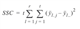
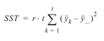
A necessary assumption in Latin-Square experiments is that there are no interactions between treatments and the row and column blocking factors. For data collected at a single location, the ANOVA table for a Latin-Square experiment is usually organized into five rows, see ANOVA Table for a Latin-Square Experiment at one Location.
|
SOURCE |
DF |
Sum of Squares |
Mean Squares |
|---|---|---|---|
|
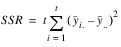
ROWS |
t – 1 |
|
MSR |
|
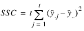
COLUMNS |
t – 1 |
|
MSC |
|
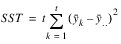
TREATMENTS |
t – 1 |
|
MST |
|
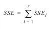
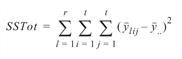
ERROR |
(t – 1)(t – 2) |
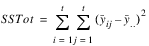
SSE=SSTot-SSR-SSC-SST |
MSE |
|
TOTAL |
t2 – 1 |
|
|
The statistical model used to represent data is from a single location:
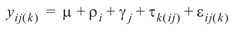
where:
yij(k) is the observation for the kth treatment in the ith row and jth column of the Latin Square.
tk(ij) is the effect associated with the kth treatment.
ri and gj are the ith row and jth column effects, respectively.
eij(k) is the noise associated with this observation.
If multiple locations are involved, LATIN_SQUARE assumes that treatments are crossed with locations, but that row and column effects are nested within locations, see ANOVA Table for a Latin-Square Experiment at Multiple Locations. The statistical model used to represent this data is:

where:
tk(ij) is the effect associated with the kth treatment
atlk(ij) is the interaction effect between location l and treatment k.

Example
This example uses four treatments organized into a latin square.
; Total number of observations
n = 16
; Number of locations
n_locations = 1
; Number of rows, columns and treatments
n_treatments = 4
col = [1, 2, 3, 4, 1, 2, 3, 4, 1, 2, 3, 4, 1, 2, 3, 4]
row = [3, 2, 4, 1, 1, 4, 2, 3, 2, 3, 1, 4, 4, 1, 3, 2]
treatment = [1, 1, 1, 1, 2, 2, 2, 2, 3, 3, 3, 3, 4, 4, 4, 4]
y = [1.167, 1.185, 1.655, 1.345, 1.64 , 1.29, 1.665, 1.29, $
1.475, 0.71, 1.425, 0.66, 1.565, 1.29, 1.4 , 1.18]
aov = LATIN_SQUARE(n, n_locations, n_treatments, row, col, $
treatment, y, cv=cv, $
treatment_means=treatment_means, $
std_err=std_err, $
grand_mean=grand_mean, $
anova_row_labels=anova_row_labels)
PRINT, "*** Experimental Design ***"
PRINT, "========================"
PRINT, "|COL | 1 | 2 | 3 | 4 |"
PRINT, "========================"
PRINT, "|ROW 1 | 2 | 4 | 3 | 1 |"
PRINT, "========================"
PRINT, "|ROW 2 | 3 | 1 | 2 | 4 |"
PRINT, "========================"
PRINT, "|ROW 3 | 1 | 3 | 4 | 2 |"
PRINT, "========================"
PRINT, "|ROW 4 | 4 | 2 | 1 | 3 |"
PRINT, "========================"
PRINT, ''
; Print Analysis of Variance Table
PRINT, " *** ANALYSIS OF VARIANCE TABLE ***"
PRINT, 'ID', 'DF', 'SSQ', 'MS', 'F-test', 'P-Value', $
Format='(A27, A5, A7, A6, A8, A8)' & $
FOR i=0L, (SIZE(aov))(1)-1 DO $
PRINT, anova_row_labels(i), aov(i,0), aov(i,1), $
aov(i,2), aov(i,3), aov(i,4), aov(i,5), Format= $
'(A23, 1X, I3, 2X, F3.0, 1X, F6.2, 1X, F6.2, 2X, ' + $
'F5.2, 2X, F6.3)'
PRINT, ''
PRINT, grand_mean, $
Format='("Grand Mean :", F7.3)'PRINT, cv, Format='("Coefficient of Variation:", F7.3)'PRINT, ''
PRINT, "Treatment Means:"
FOR i=0L, n_treatments-1 DO $
PRINT, (i+1), treatment_means(i), Format= $
"(2X, 'Treatment[', I1, '] Mean:', F7.4)"
PRINT, ''
PRINT, std_err(0), Format='("Standard Error for ' + $'Comparing Two Treatment Means: ", F8.6, I1)'
PRINT, FIX(std_err(1)), Format='("(df=", I1, ")")'PRINT, ''
; Perform multiple comparison using the LSD procedure
equal_means = MULTICOMP(treatment_means, std_err(1), $
std_err(0)/SQRT(2.0), $
/LSD, Alpha=0.05)
PM, equal_means, $
Title="LSD Comparison: Size of Groups of Means"
Output
*** Experimental Design ***
========================
|COL | 1 | 2 | 3 | 4 |
========================
|ROW 1 | 2 | 4 | 3 | 1 |
========================
|ROW 2 | 3 | 1 | 2 | 4 |
========================
|ROW 3 | 1 | 3 | 4 | 2 |
========================
|ROW 4 | 4 | 2 | 1 | 3 |
========================
*** ANALYSIS OF VARIANCE TABLE ***
ID DF SSQ MS F-test P-Value
Locations ............. -1 NaN NaN NaN NaN NaN
Rows within Locations . -2 3. 0.18 0.06 2.06 0.207
Columns within Location -3 3. 0.59 0.20 6.58 0.025
Treatments ............ -4 3. 0.35 0.12 3.93 0.073
Locations x Treatments -5 NaN NaN NaN NaN NaN
Error within Locations -6 6. 0.18 0.03 NaN NaN
Corrected Total ....... -7 15. 1.31 NaN NaN NaN
Grand Mean : 1.309
Coefficient of Variation: 13.204
Treatment Means:
Treatment[1] Mean: 1.3380
Treatment[2] Mean: 1.4712
Treatment[3] Mean: 1.0675
Treatment[4] Mean: 1.3587
Standard Error for Comparing Two Treatment Means: 0.122202
(df=6)
LSD Comparison: Size of Groups of Means
3
3
0


