LINPROG Function
Solves a linear programming problem using the revised simplex algorithm.
Usage
result = LINPROG(a, b, c)
Input Parameters
a—Two-dimensional matrix containing the coefficients of the constraints. The coefficient for the ith constraint is contained in A (i, *).
b—One-dimensional matrix containing the right-hand side of the constraints. If there are limits on both sides of the constraints, b contains the lower limit of the constraints.
c—One-dimensional array containing the coefficients of the objective function.
Returned Value
result—The solution x of the linear programming problem.
Input Keywords
Double—If present and nonzero, double precision is used.
Bu—Array with N_ELEMENTS(b) elements containing the upper limit of the constraints that have both the lower and the upper bounds. If no such constraint exists, Bu is not needed.
Irtype—Array with N_ELEMENTS(b) elements indicating the types of general constraints in the matrix A. Let ri = Ai0x0 + ... + Ain–1 xn–1. The value of Irtype (i) is described in Constraint Types.
|
Irtype (i) |
Constraints |
|
0 |
ri = bi |
|
1 |
ri £ bu |
|
2 |
ri ³ bi |
|
3 |
bi £ ri £ bu |
Default: Irtype (*) = 0
Xlb—Array with N_ELEMENTS(c) elements containing the lower bound on the variables. If there is no lower bound on a variable, 1030 should be set as the lower bound. Default: Xlb (*) = 0
Xub—Array with N_ELEMENTS(c) elements containing the upper bound on the variables. If there is no upper bound on a variable, –1030 should be set as the upper bound. Default: Xub (*) = infinity
Itmax—Maximum number of iterations. Default: Itmax = 10,000
Output Keywords
Obj—Name of the variable into which the optimal value of the objective function is stored.
Dual—Name of the variable into which the array with N_ELEMENTS(c) elements, containing the dual solution, is stored.
Discussion
Function LINPROG uses a revised simplex method to solve linear programming problems; i.e., problems of the form:

subject to:
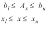
where c is the objective coefficient vector, A is the coefficient matrix, and the vectors bl, bu, xl, and xu are the lower and upper bounds on the constraints and the variables.
For a complete discussion of the revised simplex method, see Murtagh (1981) or Murty (1983). This problem can be solved more efficiently.
Example
The linear programming problem in the standard form:
min f(x) = –x0 – 3x1
subject to:
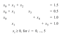
is solved.
; Define the coefficients of the constraints.
RM, a, 4, 6
1 1 1 0 0 0
1 1 0 -1 0 0
1 0 0 0 1 0
0 1 0 0 0 1
; Define the right-hand side of the constraints.
RM, b, 4, 1
1.5
.5
1
1
; Define the coefficients of the objective function.
RM, c, 6, 1
-1
-3
0
0
0
0
; Call LINPROG and print the solution.
PM, LINPROG(a, b, c), Title = 'Solution'
; PV-WAVE prints the following:
; Solution
; 0.500000
; 1.00000
; 0.00000
; 1.00000
; 0.500000
; 0.00000
Warning Errors
MATH_PROB_UNBOUNDED—Problem is unbounded.
MATH_TOO_MANY_ITN—Maximum number of iterations exceeded.
MATH_PROB_INFEASIBLE—Problem is infeasible.
Fatal Errors
MATH_NUMERIC_DIFFICULTY—Numerical difficulty occurred. If float is currently being used, using double may help.
MATH_BOUNDS_INCONSISTENT—Bounds are inconsistent.


