HOMOGENEITY Function
Conducts Bartlett’s and Levene’s tests of the homogeneity of variance assumption in analysis of variance.
Usage
result = HOMOGENEITY (n_treatment, treatment, y)
Input Parameters
n_treatment—Number of treatments. n_treatment must be greater than one.
treatment—Array of length n, where n is the number of observations, containing the treatment identifiers for each observation in y. Each level of the treatment must be assigned a different integer. HOMOGENEITY verifies that the number of unique treatment identifiers is equal to n_treatment.
y—Array of length n, where n is the number of observations, containing the experimental observations and any missing values. Missing values cannot be omitted. They are indicated by placing a NaN (Not a Number) at the appropriate positions in y. NaN can be defined by calling the MACHINE function. For example:
x = MACHINE(/Float)
y(i) = x.NaN
Returned Value
result—A 2 element array containing the p-values for Bartletts and Levene’s tests.
Input Keywords
Double—If present and nonzero, double precision is used.
Median_levenes—If set and nonzero, Levene's test is calculated using treatment medians. By default, treatment means are used.
Output Keywords
N_missing—Number of missing values, if any, found in y. Missing values are denoted with a NaN (Not a Number) value in y. In these analyses, any missing values are ignored.
Cv—The coefficient of variation computed using the grand mean and pooled within treatment standard deviation.
Grand_mean—Mean of all the data across every location.
Treatment_means—Array of size n_treatment containing the treatment means.
Residuals—Array of length n containing the residuals for non-missing observations. The ordering of the values in this array corresponds to the ordering of values in y and identified by the values in treatment.
Studentized_residuals—Array of length n containing the studentized residuals for non-missing observations. The ordering of the values in this array corresponds to the ordering of values in y and identified by the values in treatment.
Std_devs—Array of length n_treatment containing the treatment standard deviations.
Bartletts—Test statistic for Bartlett’s test.
Levenes—Test statistic for Levene’s test.
Discussion
Traditional analysis of variance assumes that variances within treatments are equal. This is referred to as homogeneity of variance. HOMOGENEITY conducts both the Bartlett’s and Levene’s tests for this assumption:

versus:

for at least one pair (i ≠ j), where t = n_treatments.
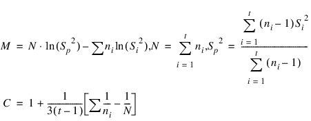
Bartlett’s test, Bartlett (1937), uses the test statistic:

where:

and  is the variance of the
  non-missing observations in the ith treatment.
  is referred to as the pooled variance, and it is also known as the error mean squares from a 1-way analysis of variance.
 is the variance of the
  non-missing observations in the ith treatment.
  is referred to as the pooled variance, and it is also known as the error mean squares from a 1-way analysis of variance.
If the usual assumptions associated with the analysis of variance are valid, then Bartlett’s test statistic is a chi-squared random variable with degrees of freedom equal to t – 1.
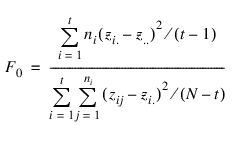
The original Levene’s test, Levene (1960) and Snedecor & Cochran (1967), uses a different test statistic, F0, equal to:

where:

 is the jth observation from the ith treatment and
  is the mean for the ith treatment. Conover, Johnson, and Johnson (1981) compared over 50 similar tests for homogeneity and concluded that one of the best tests was Levene’s test when the treatment mean,
  is replaced with the treatment median,
  . This version of Levene’s test can be requested by setting the Median_levenes keyword. In either case, Levene’s test statistic is treated as a F random variable with numerator degrees of freedom equal to (t – 1) and denominator degrees of freedom (N – t).
The residual for the jth observation within the ith treatment,  , returned from Residuals is unstandarized, i.e.
  . For investigating problems of homogeneity of variance, the studentized residuals returned by Studentized_residuals are recommended since they are standardized by the standard deviation of the residual. The formula for calculating the studentized residual is:
 , returned from Residuals is unstandarized, i.e.
  . For investigating problems of homogeneity of variance, the studentized residuals returned by Studentized_residuals are recommended since they are standardized by the standard deviation of the residual. The formula for calculating the studentized residual is:
where the coefficient of variation, returned from cv, is also calculated using the pooled variance and the grand mean  :
:
 :
:
Example
This example applies Bartlett’s and Levene’s test to verify the homogeneity assumption for a one-way analysis of variance. There are eight treatments, each with 3 replicates for a total of 24 observations. The estimated treatment standard deviations range from 5.35 to 13.17.
In this case, Bartlett's test is not statistically significant for a stated significance level of 0.05; whereas Levene's test is significant with p = 0.006.
n = 24
n_treatment = 8
treatment = [1, 2, 3, 4, 5, 6, 7, 8, $
1, 2, 3, 4, 5, 6, 7, 8, $
1, 2, 3, 4, 5, 6, 7, 8]
y = [30.0, 40.0, 38.9, 38.2, $
41.8, 52.2, 54.8, 58.2, $
20.5, 26.9, 21.4, 25.1, $
26.4, 36.7, 28.9, 35.9, $
21.0, 25.4, 24.0, 23.3, $
34.4, 41.0, 33.0, 34.9]
pv = HOMOGENEITY(n_treatment, treatment, y, $
/Median_Levenes, $
N_missing=n_missing, $
Grand_mean=grand_mean,$
Cv=cv, $
Treatment_means=treatment_means, $
Residuals=residuals, $
Studentized_residuals=studentized_residuals, $
Std_devs=std_devs, $
Bartletts=bartletts, $
Levenes=levenes)
PRINT, '*** Bartlett''s Test ***'
PRINT, ''
PRINT, pv(0), Format='("Bartlett''s p-value = ", F7.3)'PRINT, bartletts, Format='("Bartlett''s test statistic = ", $F7.3)'
PRINT, ''
PRINT, ''
PRINT, '*** Levene''s Test ***'
PRINT, ''
PRINT, pv(1), Format='("Levene''s p-value = ", F7.3)'PRINT, levenes, Format='("Levene''s test statistic = ", F7.3)'PRINT, ''
PRINT, 'Treatment means' & PRINT, treatment_means, $
Format='(F8.2)'
PRINT, ''
PRINT, 'Treatment std devs' & PRINT, std_devs, Format='(F8.2)'
PRINT, ''
PRINT, grand_mean, Format='("grand_mean = ", F7.3)'PRINT, cv, Format='("cv = ", F7.3)'PRINT, n_missing, Format='("n_missing = ", I3)'Output
*** Bartlett's Test ***
Bartlett's p-value = 0.944
Bartlett's test statistic = 2.257
*** Levene's Test ***
Levene's p-value = 0.994
Levene's test statistic = 0.135
Treatment means
23.83
30.77
28.10
28.87
34.20
43.30
38.90
43.00
Treatment std devs
5.35
8.03
9.44
8.13
7.70
8.00
13.92
13.17
grand_mean = 33.871
cv = 28.378
n_missing = 0


