SP_CG Function
Solves a real symmetric definite linear system using a conjugate gradient method. Using keywords, a preconditioner can be supplied.
Usage
result = SP_CG(amultp, b)
Input Parameters
amultp—Scalar string specifying a user supplied function which computes z = Ap. The function accepts the argument p, and returns the vector Ap.
b—One-dimensional matrix containing the right-hand side.
Returned Value
result—A one-dimensional array containing the solution of the linear system Ax = b.
Input Keywords
Precond—Scalar string specifying a user supplied function which sets z = M –1r, where M is the preconditioning matrix.
Jacobi—If present, use the Jacobi preconditioner, that is, M = diag(A). The user-supplied vector Jacobi should be set so that jacobi(i) = Ai,i.
Double—If present and nonzero, double precision is used.
Input/Output Keywords
Itmax—Initially set to the maximum number of GMRES iterations allowed. On exit, the number of iterations used is returned. Default: Itmax = 1000
Rel_err—Initially set to relative error desired. On exit, the computed relative error is returned. Default: Rel_err = SQRT(machine precision)
Discussion
The function SP_CG solves the symmetric definite linear system Ax = b using the conjugate gradient method with optional preconditioning. This method is described in detail by Golub and Van Loan (1983, chapter 10), and in Hageman and Young (1981, chapter 7).
The preconditioning matrix M, is a matrix that approximates A, and for which the linear system Mz = r is easy to solve. These two properties are in conflict; balancing them is a topic of much current research. In the default usage of SP_CG, M = I. If the keyword Jacobi is selected, M is set to the diagonal of A.
The number of iterations needed depends on the matrix and the error tolerance. As a rough guide:
 for
for 
See the academic references for details.
Let M be the preconditioning matrix, let b, p, r, x, and z be vectors and let t be the desired relative error. Then the algorithm used is as follows:


Here λ is an estimate of λmax(G), the largest eigenvalue of the iteration matrix G = I – M–1A. The stopping criterion is based on the result (Hageman and Young, 1981, pages 148-151):

where  . It is also known that:
 . It is also known that:
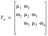
where the  are the symmetric, tridiagonal matrices:
 are the symmetric, tridiagonal matrices:
with μk = 1 – βk/αk–1, μ1 = 1 – 1/α1, and ωk = SQRT(βk)/αk–1. Usually the eigenvalue computation is needed for only a few of the iterations.
Example 1
In this example, the solution to a linear system is found. The coefficient matrix is stored as a full matrix.
; Since A is in dense form, we use the # operator to perform the
; matrix-vector product. The common block us used to hold A.
FUNCTION Amultp, p
COMMON Cg_comm1, a
RETURN, a#p
END
Pro CG_EX1
COMMON Cg_comm1, a
a = TRANSPOSE([[ 1, -3, 2], [-3, 10, -5], [ 2, -5, 6]])
b = [27, -78, 64]
x = SP_CG('amultp', b); Use SP_CG to compute the solution, then output the result.
PM, x, title = 'Solution to Ax = b'
END
; Output of this procedure:
;
; Solution to Ax = b
; 1.0000000
; -4.0000000
; 7.0000000
See Also


