This section introduces some of the mathematical concepts used with PV‑WAVE.

Function INV is used to invert an n × n nonsingular matrix—either real or complex. The inverse also can be obtained by using keyword Inverse in functions for solving systems of linear equations. The inverse of a matrix need not be computed if the purpose is to solve one or more systems of linear equations. Even with multiple right-hand sides, solving a system of linear equations by computing the inverse and performing matrix multiplication is usually more expensive than the method discussed in the next section.

A square system of linear equations has the form Ax = b, where A is a user-specified n × n matrix, b is a given n-vector, and x is the solution n-vector. Each entry of A and b must be specified by the user. The entire vector x is returned as output.

When A is invertible, a unique solution to Ax = b exists. The most commonly used direct method for solving Ax = b factors the matrix A into a product of triangular matrices and solves the resulting triangular systems of linear equations. Functions that use direct methods for solving systems of linear equations all compute the solution to Ax = b. PV‑WAVE IMSL Mathematics functions LUSOL, CHSOL, and CHNNDSOL can be used to compute x.

In some applications, you may only want to factor the n × n matrix A into a product of two triangular matrices. Functions and procedures that end with “FAC” are designed to compute these factorizations. Suppose that in addition to the solution x of a linear system of equations Ax = b, you want the LU factorization of A. First, use the LUFAC procedure to obtain the LU factorization in a condensed format; then, call LUSOL with this factorization and a right-hand side b to compute the solution. If the factorization is desired in separate, full matrices, the LUFAC procedure can be called with keywords L and U to return L and U separately.

Besides the basic matrix factorizations, such as LU and LLT, additional matrix factorizations also are provided. For a real matrix A, QR factorization can be computed by the QRFAC procedure. Functions for computing the Singular Value Decomposition (SVD) of a matrix are discussed in a later section.

Consider the case in which a system of linear equations has more than one right-hand side vector. It is most economical to find the solution vectors by first factoring the coefficient matrix A into products of triangular matrices. Then, the resulting triangular systems of linear equations are solved for each right-hand side. When A is a real general matrix, access to the LU factorization of A is computed by using the LUFAC procedure. The solution xk for the k-th right-hand side vector bk is then found by two triangular solves, Lyk = bk and Uxk = yk. The LUSOL function is called with the computed factorization and is used to solve each right-hand side. This process can be followed when using other functions for solving systems of linear equations.

Least-squares solutions are usually computed for an over-determined system of linear equations Am × n x = b, where m > n. A least-squares solution x minimizes the Euclidean length of the residual vector r = Ax – b. The QRSOL function computes a unique least-squares solution for x when A has full-column rank. If A is rank-deficient, then the base solution for some variables is computed. These variables consist of the resulting columns after the interchanges. The QR decomposition, with column interchanges or pivoting, is computed such that AP = QR. Here, Q is orthogonal, R is upper-trapezoidal with its diagonal elements nonincreasing in magnitude, and P is the permutation matrix determined by the pivoting. The base solution xB is obtained by solving R(PT)x = QTb for the base variables. For details, see the Discussion of the QRSOL Function. The QR factorization of a matrix A, such that AP = QR with P specified by the user, can be computed using the QRFAC procedure.

The SVD of an m by n matrix A is a matrix decomposition, A = USVT. With
q = min(m, n), the factors Um × q and Vn × q are orthogonal matrices, and Sq × q is a nonnegative diagonal matrix with nonincreasing diagonal terms. The SVDCOMP function computes the singular values of A by default. By using keywords, part or all of the U and V matrices, an estimate of the rank of A, and the generalized inverse of A also can be obtained.

An m × n matrix A is mathematically singular if an x ≠ 0 exists such that Ax = 0. In this case, the system of linear equations Ax = b does not have a unique solution. However, a matrix A is numerically singular if it is “close” to a mathematically singular matrix. Such problems are called ill-conditioned. If the numerical results with an ill-conditioned problem are unacceptable, either use more accuracy if available (for type float switch to double) or obtain an approximate solution to the system. One form of approximation can be obtained using the SVD of A: If q = min(m, n) and:

then the approximate solution is given by the following:

The scalars ti,i are defined by:

The user specifies the value of tol. This value determines how “close” the given matrix is to a singular matrix. Further restrictions may apply to the number of terms in the sum, k ≤ q. For example, there may be a value of k ≤ q such that the scalars | (bTui)|, i > k, are smaller than the average uncertainty in the right-hand side b. This means that these scalars can be replaced by zero, and hence, b is replaced by a vector that is within the stated uncertainty of the problem.

Since many functions and procedures described in this chapter operate on both real or complex matrices, the notation AH is used to represent both the transpose of A if A is real and the conjugate transpose if A is complex.

A number of routines employ direct methods (as opposed to iterative methods) for solving problems involving sparse matrices.

For general sparse linear systems, SP_LUFAC and SP_LUSOL form a factor/solve function pair. If a sparse matrix the problem Ax = b is to be solved for a single A, but multiple right-hand sides, b, then SP_LUFAC should first be used to compute an LU decomposition of A, then follow multiple calls to SP_LUSOL (one for each right-hand side, b). If only one right-hand side, b, is involved then SP_LUSOL can be called directly, in which case the factor step is computed internally by SP_LUSOL.

For general banded systems, SP_BDSOL and SP_BDFAC form a factor/solve pair. The relationship between SP_BSFAC and SP_BDSOL is similar to that of SP_LUFAC and SP_LUSOL.

The functions SP_PDFAC and SP_PDSOL are provided for working with systems involving sparse symmetric positive definite matrices. The relationship between SP_PDFAC and SP_PDSOL is similar to that of SP_LUFAC and SP_LUSOL.

The functions SP_BDDFAC and SP_BDPDSOL are provided for working with systems involving banded symmetric positive definite matrices. The relationship between SP_BDPDFAC and SP_BDPDSOL is similar to that of SP_LUFAC and SP_LUSOL.

Two routines are provided that employ iterative methods (as opposed to direct methods) for solving problems involving sparse matrices.

The function SP_GMRES, based on the FORTRAN subroutine GMRESD by H. F. Walker, solves the linear system Ax = b using the GMRES method. This method is described in detail by Saad and Schultz (1986) and Walker (1988).

The function SP_CG solves the symmetric definite linear system Ax = b using the conjugate gradient method with optional preconditioning. This method is described in detail by Golub and Van Loan (1983, chapter 10), and in Hageman and Young (1981, chapter 7).

Utilities designed to aid with the manipulation of sparse matrices are also provided. The common operation of matrix-vector multiplication can be efficiently executed using the function SP_MVMUL.

The dense linear algebra functions in PV‑WAVE require input consisting of matrix dimensions and all values for the matrix entries. Clearly, this is not practical for sparse linear algebra. Three different storage formats can be used for the functions in the sparse matrix sections. These methods include:

Only the non-zero elements of a sparse matrix need to be communicated to a function. Sparse coordinate storage format stores the value of each matrix entry along with that entry’s row and column index. The following system variables are defined to support this concept:

!F_SP_ELEM = {f_sp_elem_str, row:0L, col:0L, val:float(0.0)}

!D_SP_ELEM = {d_sp_elem_str, row:0L, col:0L, val:double(0.0)}

!C_SP_ELEM = {c_sp_elem_str, row:0L, col:0L, val:complex(0.0)}

!Z_SP_ELEM = {z_sp_elem_str, row:0L, col:0L, val:dcomplex(0.0)}

As an example consider the 6 × 6 matrix:

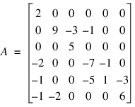
The matrix A has 15 non-zero elements, and its sparse coordinate representation would be:

Since this representation does not rely on order, an equivalent form would be:

There are different ways this data could be used to initialize. Consider the following program fragment:

A = replicate(!F_sp_elem, 15)

a(*).row = [0, 1, 1, 1, 2, $

            3, 3, 3, 4, 4, $

            4, 4, 5, 5, 5]

a(*).col = [0, 1, 2, 3, 2, $

            0, 3, 4, 0, 3, $

           4, 5, 0, 1, 5]

a(*).val = [2, 9, -3, -1, 5,$

            -2, -7, -1, -1, -5, 1, $

            -3, -1, -2, 6]

B = replicate(!F_sp_elem, 15)

b(*).row = [5, 4, 3, 0, 5, $

            1, 2, 1, 4, 3, $

            1, 4, 3, 5, 4]

b(*).col = [0, 0, 0, 0, 1, $

            1, 2, 2, 3, 3, $

            3, 4, 4, 5, 5]

b(*).val = [-1, -1, -2, 2, -2,$

            9, 5, -3, -5, -7, -1, $

            1, -1, 6, -3]

Both a and b represent the sparse matrix A.

A sparse symmetric or Hermitian matrix is a special case, since it is only necessary to store the diagonal and either the upper or lower triangle. As an example, consider the 5 × 5 linear system:

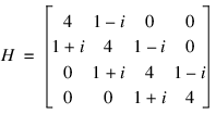
The Hermitian and symmetric positive definite system solvers in this module expect the diagonal and lower triangle to be specified. The sparse coordinate form for the lower triangle is given by

The following program fragment will initialize H.

A = replicate(!C_sp_elem, 7)

a(*).row = [0, 1, 2, 3, 1, 2, 3]

a(*).col = [0, 1, 2, 3, 0, 1, 2]

a(*).val = [COMPLEX(4, 0), COMPLEX(4, 0), $

            COMPLEX(4, 0), COMPLEX(4, 0), $

            COMPLEX(1, 1), COMPLEX(1, 1), $

            COMPLEX(1, 1)] 

There are some important points to note here. Note that H is not symmetric, but rather Hermitian. The functions that accept Hermitian data understand this and operate assuming that:

The Sparse Matrix Module cannot take advantage of the symmetry in matrices that are not positive definite. The implication here is that a symmetric matrix that happens to be indefinite cannot be stored in this compact symmetric form. Rather, both upper and lower triangles must be specified and the sparse general solver called.

A band matrix is an M × N matrix A with all of its non-zero elements “close” to the main diagonal. Specifically, values Aij = 0 if i – j > nlca or j – i > nuca. The integer m = nlca + nuca + 1 is the total band width. The diagonals, other than the main diagonal, are called codiagonals. While any M × N matrix is a band matrix, band storage format is only useful when the number of non-zero codiagonals is much less than N.

In band storage format, the nlca lower codiagonals and the nuca upper codiagonals are stored in the rows of an array of size m × N. The elements are stored in the same column of the array as they are in the matrix. The values Aij inside the band width are stored in the linear array in positions ((i-j+nuca+1)* n+j). This results in a row-major, one-dimensional mapping from the two-dimensional notion of the matrix.

For example, consider the 5 × 5 matrix A with 1 lower and 2 upper codiagonals:

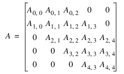
In band storage format, the data would be arranged as:

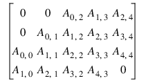
This data would be then be stored contiguously, row-major order, in an array of length 20.

As an example, consider the following tridiagonal matrix:

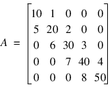
The following code segment will store this matrix in band storage format:

a = [0, 1, 2, 3, 4, $

     10, 20, 30, 40, 50, $

     5, 6, 7, 8, 0]

As in the sparse coordinate representation, there is a space saving symmetric version of band storage. As an example, we look at the following 5 × 5 symmetric problem:

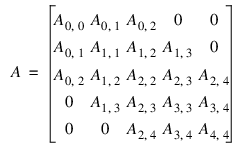
In band symmetric storage format, the data would be arranged as:

The following Hermitian example illustrate the procedure:

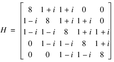
The following program fragments stores H in h, using band symmetric storage format:

h = complexarr(15)

h(0:1) = 0

h(2:4) = complex(1,1)

h(5) = 0

h(6:9) = complex(1,1)

h(10:14) = 8

It is clear that any matrix can be stored in either sparse coordinate or band format. The choice depends on the sparsity pattern of the matrix. A matrix with all non-zero data stored in bands close to the main diagonal would probably be a good candidate for band format. If non-zero information is scattered more or less uniformly through the matrix, sparse coordinate format is the best choice. As extreme examples, consider the following two cases. First, consider an n × n matrix with all elements on the main diagonal and the (0,n–1) and (n–1,0) entries non-zero. The sparse coordinate vector would be n + 2 units long. An array of length 2n2 – n would be required to store the band representation, nearly twice as much storage as a dense solver might require. Secondly, consider a tridiagonal matrix with all diagonal, superdiagonal and subdiagonal entries non-zero. In band format, an array of length 3n is needed. In sparse coordinate format, a vector of length 3n – 2 is required. But the problem is that, for instance with floating-point precision on a 32 bit machine, each of those 3n – 2 units in coordinate format requires three times as much storage as any of the 3n units needed for band representation. This is due to carrying the row and column indices in coordinate form. Band storage evades this requirement by being essentially an ordered list, and defining location in the original matrix by position in the list.

Functions that accept data in coordinate format can also accept data stored in the format described in the Users’ Guide for the Harwell-Boeing Sparse Matrix Collection. The scheme is column oriented, with each column held as a sparse vector, represented by a list of the row indices of the entries in an integer array and a list of the corresponding values in a separate float (double, complex, dcomplex) array. Data for each column are stored consecutively and in order. A separate integer array holds the location of the first entry of each column and the first free location. Only entries in the lower triangle and diagonal are stored for symmetric and Hermitian matrices. All arrays are based at zero, which is in contrast to the Harwell-Boeing test suite’s one-based arrays.

As in the Harwell-Boeing Users’ Guide, we illustrate the storage scheme with the following example. The 5x5 matrix:

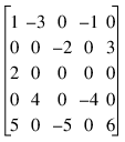
would be stored in the arrays colptr (location of first entry), rowind (row indices), and values (non-zero entries) as follows: