PDE_1D_MG Procedure (PV-WAVE Advantage)
Solves a system of partial differential equations of the form:
where:
 m
m is 0, 1, or 2
 t ≥ t0
 and
xL ≤ x ≤ xR are scalars
 u
u(
t,
x) is the n-element solution vector
 r
r(
t,x,u,∂ u/∂ x) and
q(
t,x,u,∂ u/∂ x) are n-element vectors
 C
C(
t,x,u,∂ u/∂ x) is an (
n,
n) matrix
Usage
pde_1d_mg, ti, xji, ujki, evalcqr, evalbcs
Input Parameters
ti—A p-element array of t values at which to solve for u(t,x). The values must be monotonically increasing or decreasing. ti(0) is the intial value.
xji—A q-element array of x values at which u(ti(0), x) is known. The values must be monotonically increasing.
ujki—A (q,n) array specifying the initial values u(ti(0), xji).
evalcqr—A user-supplied procedure to evaluate c, q, and r. Its parameter list is t, x, uall, uloc, dudx, c, q, r, err. All are inputs and the last four are outputs. t and x are scalar values of the independent variables. uall is a (q,n+1) array where uall(*,n) increases from xji(0) to xji(q–1) and where uall(*,0:n–1) approximates u(t,uall(*,n)). uloc and dudx are n-element arrays approximating u(t,x) and (∂ u/∂ x)(t,x). c, q, and r have been previously defined. The scalar err should be changed to 3 if an error occurs. All floating point input will be double precision and all output must be of type double precision.
evalbcs—A user-supplied procedure to evaluate boundary conditions. The parameter list is t, left, uall, uloc, dudx, beta, gamma, err. All are inputs and the last three are outputs. t is a scalar. If left = 1, the left boundary condition must be evaluated and if left = 0 the right boundary condition must be evaluated. The values uall, uloc, and dudx are arrays as previously defined for evalcqr. beta(t,x,u,∂ u/∂ x) and gamma(t,x,u,∂ u/∂ x) are n-element arrays defining boundary conditions as betairi = gammai, where i=0, ..., n–1 and r has been previously defined. The scalar err should be changed to 3 if an error occurs. All floating point input will be double precision and all output must be of type double precision.
Output Parameters
xji—A (q,p) array of x values. xji(*,i) contains the x values at which the solution has been computed for ti(i). The value xji(*,i) is increasing and covers the same range as initial grid xji(*,0). The default grid is distributed so that density increases with |∂ u/∂ x|, but other distributions are possible with keywords.
ujki—A (q,n,p) array containing the solution. ujki(j,*,i) = u(ti(i), xji(j,i))
Input Keywords
M—The integer from the differential equation above. The default of 0 is for problems in cartesian coordinates, while a value of 1 or 2 is for problems in coordinates which are cylindrical or spherical respectively. In the latter cases t is the angle around the z-axis and x is the radial variable which must not contain 0 in the interior of its range.
Tau—A scalar ≥ 0 control on grid line smoothing (see the Discussion section). The default is 0, but higher values may be needed to prevent oscillating or crossing grid lines. A large value results in straight and evenly spaced gridlines.
Kappa—A scalar ≥ 0 control on grid line smoothing (see the Discussion section). The default is 2, and lower values decrease smoothing.
Alpha—A scalar ≥ 0 control on grid line smoothing (see the Discussion section). The default is 0.01.
Bdf_order_max—Integer upper limit on the order of backward difference formula used for t derivatives. The default is 2.
User_factor_solve—A 2-element array of names of procedures that factor and solve the linear system associated with integration in the
t direction (see the
Discussion section and
DEA_PETZOLD_GEAR Procedure (PV-WAVE Advantage)).
User_factor_solve(0) has parameter list
iband,
b,
err.
iband and
b are inputs where
b is a (
n, 2*
iband+1) array representing an (
n,
n) banded matrix in band storage mode. The procedure factors
b or checks its condition number.
err is output as zero for success or nonzero for failure. Any factorization is stored in a common block shared by
User_factor_solve(1), which in turn has parameter list
iband,
g,
y.
iband is input as above, and
g is input as an n-element array.
y is output as an n-element array solution to the linear system
by =
g. All floating point input will be double precision and
all output must be of type double precision.
Rtol—A scalar relative accuracy required from the integrator
DEA_PETZOLD_GEAR Procedure (PV-WAVE Advantage). The default is 1e–4.
Atol—A scalar absolute accuracy required from the integrator
DEA_PETZOLD_GEAR Procedure (PV-WAVE Advantage). The default is 1e–4.
Example 1: Electrodynamics Model
This example is from Blom and Zegeling (1994). The system is:
ut = ε puxx – g(u – v)
vt = pvxx + g(u – v)
where g(z) = exp(η z/3) – exp(–2η z/3)
0 ≤ x ≤ 1, 0 ≤ t ≤ 4
ux = 0 and v = 0 at x = 0
u = 1 and vx = 0 at x = 1
ε = 0.143, p = 0.1743, η = 17.19
We make the connection between the model problem statement and the example:
C = I2
m = 0, R1 = ε pux, R2 = pvx
Q1 = g(u – v), Q2 = –Q1
u = 1 and v = 0 at t = 1
The boundary conditions are:
β1 = 1, β2 = 0, γ 1 = 0, γ 2 = v, at x = xL = 0
β1 = 0, β2 = 1, γ 1 = u – 1, γ 2 = 0, at x = xR = 1
This is a non-linear problem with sharply changing conditions near t = 0. The default settings of integration parameters allow the problem to be solved. The use of PDE_1D_MG requires two subroutines provided by the user to describe the differential equations, and boundary conditions.
The full example is available in <RW_DIR>/wave/lib/user/examples/pde_1d_mg_ex.pro.
note | This example uses a custom procedure, PLOTEXMP, that is not included here. The file, pde_1d_mg_ex.pro, includes the code to define this procedure. |
The code for this example is:
PRO pde_systems1, t, x, full_u, grid_u, dudx, c, q, r, ires
eps = 0.143d
eta = 17.19d
pp = 0.1743d
c(0,0) = 1
c(0,1) = 0
c(1,0) = 0
c(1,1) = 1
r(0) = pp * dudx(0) * eps
r(1) = pp * dudx(1)
z = eta * (grid_u(0)-grid_u(1))/3
q(0) = EXP(z) - EXP(-2*z)
q(1) = -q(0)
END
PRO bc1, t, left, full_u, grid_u, dudx, beta, gamma, ires
IF left THEN BEGIN
beta(0) = 1
beta(1) = 0
gamma(0) = 0
gamma(1) = grid_u(1)
ENDIF ELSE BEGIN
beta(0) = 0
beta(1) = 1
gamma(0) = grid_u(0) - 1
gamma(1) = 0
ENDELSE
END
PRO pde_1d_mg_ex1, Nopl=nopl
ti = [ 0, 0.001d, 0.01d, 0.1d, 1, 4 ]
xji = INTERPOL( [0,1d], 51 )
ujki = REBIN( [[1],[0d]], 51, 2 )
PDE_1D_MG, ti, xji, ujki, "pde_systems1", "bc1"
SAVE, ti, xji, ujki, File='pde_1d_mg_ex1.dat'
IF N_ELEMENTS(nopl) EQ 0 THEN PLOTEXMP, ti, xji, ujki
END
Example 2: Inviscid Flow on a Plate
This example is a first order system from Pennington and Berzins, (1994). The equations are:
ut = –vx
uut = –vux + wxx
w = ux, implying that uut = –vux + uxx
Following elimination of w, there remain NPDE = 2 differential equations. The variable t is not time, but a second space variable. The integration goes from t = 0 to t = 5. It is necessary to truncate the variable x at a finite value, say xmax = xR = 25. In terms of the integrator, the system is defined by letting m = 0 and:
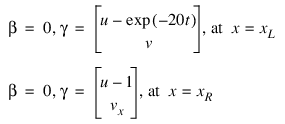
The boundary conditions are satisfied by:
We use N = 10 + 51 = 61 grid points and output the solution at steps of Δt = 0.1.
This is a non-linear boundary layer problem with sharply changing conditions near t = 0. The problem statement was modified so that boundary conditions are continuous near t = 0. Without this change the underlying integration software, DEA_PETZOLD_GEAR, cannot solve the problem. The continuous blending function u – exp(–20t) is arbitrary and artfully chosen. This is a mathematical change to the problem, required because of the stated discontinuity at t = 0. Reverse communication is used for the problem data. No additional user-written subroutines are required when using reverse communication. We also have chosen 10 of the initial grid points to be concentrated near the left boundary anticipating rapid change in the solution near that point. Optional changes are made to use a pure absolute error tolerance and non-zero time-smoothing.
The full example is available in <RW_DIR>/wave/lib/user/examples/pde_1d_mg_ex.pro.
note | This example uses a custom procedure, PLOTEXMP, that is not included here. The file, pde_1d_mg_ex.pro, includes the code to define this procedure. |
The code for this example is:
PRO pde_systems2, t, x, full_u, grid_u, dudx, c, q, r, ires
c(0,0) = 1
c(1,0) = grid_u(0)
c(0,1) = 0
c(1,1) = 0
r(0) = -grid_u(1)
r(1) = dudx(0)
q(0) = 0
q(1) = grid_u(1) * dudx(0)
END
PRO bc2, t, left, full_u, grid_u, dudx, beta, gamma, ires
beta(*) = 0
IF left THEN BEGIN
gamma(0) = grid_u(0) - EXP(-20*t)
gamma(1) = grid_u(1)
ENDIF ELSE BEGIN
gamma(0) = grid_u(0) - 1
gamma(1) = dudx(1)
ENDELSE
END
PRO pde_1d_mg_ex2, Nopl=nopl
ti = INTERPOL( [0,5d], 51 )
xji = [ INTERPOL([0,0.5d],11), INTERPOL([1,25d],49) ]
ujki = REBIN( [[1],[0d]], 60, 2 )
PDE_1D_MG, ti, xji, ujki, "pde_systems2", "bc2", $
Tau=1d-3, Atol=1d-2, Rtol=0
SAVE, ti, xji, ujki, File='pde_1d_mg_ex2.dat'
IF N_ELEMENTS(nopl) EQ 0 THEN PLOTEXMP, ti, xji, ujki
END
Example 3: Population Dynamics
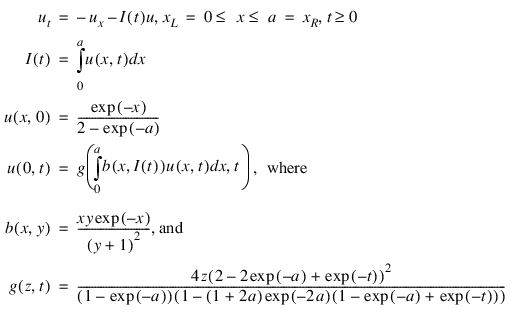
This example is from Pennington and Berzins (1994). The system is:
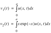
This is a notable problem because it involves the unknown:
across the entire domain. The software can solve the problem by introducing two dependent algebraic equations:
This leads to the modified system:
In the interface to the evaluation of the differential equation and boundary conditions, it is necessary to evaluate the integrals, which are computed with the values of u(x,t) on the grid. The integrals are approximated using the trapezoid rule, commensurate with the truncation error in the integrator.
This is a non-linear integro-differential problem involving non-local conditions for the differential equation and boundary conditions. Access to evaluation of these conditions is provided using common blocks. Optional changes are made to use an absolute error tolerance and non-zero time-smoothing. The time-smoothing value τ = 1 prevents grid lines from crossing.
The full example is available in <RW_DIR>/wave/lib/user/examples/pde_1d_mg_ex.pro.
note | This example uses a custom procedure, PLOTEXMP, that is not included here. The file, pde_1d_mg_ex.pro, includes the code to define this procedure. |
The code for this example is:
FUNCTION fcn_g3, z, t
a = 5d
em2a = EXP(-2*a)
ema = EXP(-a)
emt = EXP(-t)
g = 2 - 2*ema + emt
RETURN, 4*z*g*g/((1-ema)*(1-(1+2*a)*em2a)*(1-ema+emt))
END
PRO pde_systems3, t, x, full_u, grid_u, dudx, c, q, r, ires
c(0) = 1
r(0) = -grid_u
i = INTEGRAL( [(SIZE(full_u))(1)], Sur=LIST(full_u(*,1)), $
Int=full_u(*,0) )
q(0) = i * grid_u
END
PRO bc3, t, left, full_u, grid_u, dudx, beta, gamma, ires
beta(0) = 0
IF left THEN BEGIN
q = (SIZE(full_u))(1)
x = full_u(*,1)
u = full_u(*,0)
v1 = INTEGRAL( [q], Surface=LIST(x), Integrand=u )
; v2 = INTEGRAL([q], Surface=LIST(x), Integrand=x*EXP(-x)*u)
; instead of trapezoidal rule, we use midpoint rule to improve
; convergence for this problem
xr = x(1:*)
xm = 0.5d * (xr+x)
v2 = TOTAL( xm * EXP(-xm) * 0.5d*(u(1:*)+u) * (xr-x) )
gamma(0) = FCN_G3(1d,t)*v1*v2/(v1+1)^2 - grid_u
ENDIF ELSE BEGIN
gamma(0) = dudx
ENDELSE
END
PRO pde_1d_mg_ex3, Nopl=nopl
ti = INTERPOL( [0,5d], 51 )
xji = INTERPOL( [0,5d], 101 )
ujki = EXP(-xji) / (2-EXP(-MAX(xji)))
PDE_1D_MG, ti, xji, ujki, 'pde_systems3', 'bc3', Tau=1, $
Rtol=0, Atol=1d-2
SAVE, ti, xji, ujki, File='pde_1d_mg_ex3.dat'
IF N_ELEMENTS(nopl) EQ 0 THEN PLOTEXMP, ti, xji, ujki
END
Example 4: A Model in Cylindrical Coordinates
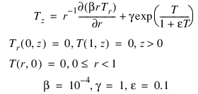
This example is from Blom and Zegeling (1994). The system models a reactor-diffusion problem:
The axial direction z is treated as a time coordinate. The radius r is treated as the single space variable.
This is a non-linear problem in cylindrical coordinates. Our example illustrates assigning m = 1.
The full example is available in <RW_DIR>/wave/lib/user/examples/pde_1d_mg_ex.pro.
note | This example uses a custom procedure, PLOTEXMP, that is not included here. The file, pde_1d_mg_ex.pro, includes the code to define this procedure. |
The code for this example is:
PRO pde_systems4, t, x, full_u, grid_u, dudx, c, q, r, ires
c(0) = 1
r(0) = 1d-4 * dudx
q(0) = -EXP(grid_u/(1+0.1d*grid_u))
END
PRO bc4, t, left, full_u, grid_u, dudx, beta, gamma, ires
IF left THEN BEGIN
beta(0) = 1
gamma(0) = 0
ENDIF ELSE BEGIN
beta(0) = 0
gamma(0) = grid_u
ENDELSE
END
PRO pde_1d_mg_ex4, Nopl=nopl
ti = INTERPOL( [0,1d], 11 )
xji = INTERPOL( [0,1d], 41 )
ujki = DBLARR(41)
PDE_1D_MG, ti, xji, ujki, 'pde_systems4', 'bc4', M=1
SAVE, ti, xji, ujki, File='pde_1d_mg_ex4.dat'
IF N_ELEMENTS(nopl) EQ 0 THEN PLOTEXMP, ti, xji, ujki
END
Example 5: A Flame Propagation Model
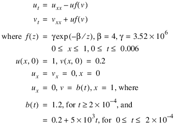
This example is presented more fully in Verwer, et al., (1989). The system is a normalized problem relating mass density u(x,t) and temperature v(x,t):
This is a non-linear problem. The example shows the model steps for replacing the banded solver in the software with one of the user’s choice. Following the computation of the matrix factorization in SP_BDFAC, we declare the system to be singular when the condition number becomes too large. This choice is not suitable for all problems. Attention must be given to detecting a singularity when this option is used.
The full example is available in <RW_DIR>/wave/lib/user/examples/pde_1d_mg_ex.pro.
note | This example uses a custom procedure, PLOTEXMP, that is not included here. The file, pde_1d_mg_ex.pro, includes the code to define this procedure. |
The code for this example is:
PRO pde_systems5, t, x, full_u, grid_u, dudx, c, q, r, ires
c(0,0) = 1
c(0,1) = 0
c(1,0) = 0
c(1,1) = 1
r(0) = dudx
q(0) = 3.52d6 * grid_u(0) * EXP(-4/grid_u(1))
q(1) = -q(0)
END
PRO bc5, t, left, full_u, grid_u, dudx, beta, gamma, ires
IF left THEN BEGIN
beta(*) = 0
gamma(0) = dudx
ENDIF ELSE BEGIN
beta(0) = [1,0]
IF t LT 2d-4 THEN BEGIN
gamma(0) = [ 0, 5d3*t+0.2-grid_u(1) ]
ENDIF ELSE BEGIN
gamma(0) = [ 0, 1.2-grid_u(1) ]
ENDELSE
ENDELSE
END
PRO fac5, iband, a, err
COMMON fac5, pivot, factor
; SP_BDFAC is used internally, but a user may substitute a
; different one
SP_BDFAC, iband, iband, (SIZE(a))(1), a(*), pivot, factor, $
Cond=c, /Doub
IF c LT 1d15 THEN err = 0d ELSE err = 1d
END
PRO sol5, iband, g, y
COMMON fac5, pivot, factor
y = SP_BDSOL( g, iband, iband, Pivot=pivot, Factor=factor, $
/Double )
END
PRO pde_1d_mg_ex5, Nopl=nopl
ti = INTERPOL( [0,0.006d], 61 )
xji = INTERPOL( [0,1d], 40 )
ujki = REBIN( [[1],[0.2d]], 40, 2 )
PDE_1D_MG, ti, xji, ujki, 'pde_systems5', 'bc5', $
Bdf_order_max=5, User_factor_solve=['fac5','sol5']
SAVE, ti, xji, ujki, File='pde_1d_mg_ex5.dat'
IF N_ELEMENTS(nopl) EQ 0 THEN PLOTEXMP, ti, xji, ujki
END
Example 6: A ‘Hot Spot’ Model
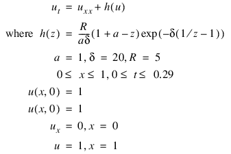
This example is presented more fully in Verwer, et al., (1989). The system is a normalized problem relating the temperature u(x,t), of a reactant in a chemical system. The formula for h(z) is equivalent to their example.
This is a non-linear problem. The output shows a case where a rapidly changing front, or hot-spot, develops after a considerable way into the integration. This causes rapid change to the grid. An option sets the maximum order BDF formula from its default value of 2 to the theoretical stable maximum value of 5.
The full example is available in <RW_DIR>/wave/lib/user/examples/pde_1d_mg_ex.pro.
note | This example uses a custom procedure, PLOTEXMP, that is not included here. The file, pde_1d_mg_ex.pro, includes the code to define this procedure. |
The code for this example is:
PRO pde_systems6, t, x, full_u, grid_u, dudx, c, q, r, ires
c(0) = 1
r(0) = dudx
q(0) = (0.25d*grid_u-0.5d) * EXP(20-20/grid_u)
END
PRO bc6, t, left, full_u, grid_u, dudx, beta, gamma, ires
beta(0) = 0
IF left THEN BEGIN
gamma(0) = dudx
ENDIF ELSE BEGIN
gamma(0) = grid_u - 1
ENDELSE
END
PRO pde_1d_mg_ex6, Nopl=nopl
ti = INTERPOL( [0,0.29d], 30 )
xji = INTERPOL( [0,1d], 80 )
ujki = REPLICATE( 1d, 80 )
PDE_1D_MG, ti, xji, ujki, 'pde_systems6', 'bc6', $
Bdf_order_max=5
SAVE, ti, xji, ujki, File='pde_1d_mg_ex6.dat'
IF N_ELEMENTS(nopl) EQ 0 THEN PLOTEXMP, ti, xji, ujki
END
Example 7: Traveling Waves
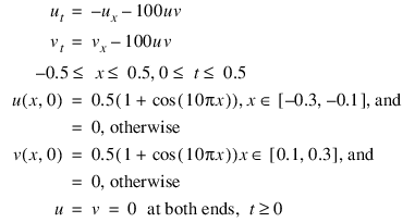
This example is presented more fully in Verwer, et al., (1989). The system is a normalized problem relating the interaction of two waves, u(x,t) and v(x,t) moving in opposite directions. The waves meet and reduce in amplitude, due to the non-linear terms in the equation. Then they separate and travel onward, with reduced amplitude.
This is a non-linear system of first order equations.
The full example is available in <RW_DIR>/wave/lib/user/examples/pde_1d_mg_ex.pro.
note | This example uses a custom procedure, PLOTEXMP, that is not included here. The file, pde_1d_mg_ex.pro, includes the code to define this procedure. |
The code for this example is:
PRO pde_systems7, t, x, full_u, grid_u, dudx, c, q, r, ires
c(0,0) = 1
c(0,1) = 0
c(1,0) = 0
c(1,1) = 1
r(0) = -grid_u(0)
r(1) = grid_u(1)
q(*) = 100 * grid_u(0) * grid_u(1)
END
PRO bc7, t, left, full_u, grid_u, dudx, beta, gamma, ires
beta(*) = 0
gamma(0) = grid_u
END
PRO pde_1d_mg_ex7, Nopl=nopl
ti = INTERPOL( [0,0.5d], 11 )
xji = INTERPOL( [-0.5d,0.5d], 50 )
ujki = DBLARR(50,2)
i0 = WHERE( -0.3d LE xji AND xji LE -0.1d )
i1 = WHERE( 0.1d LE xji AND xji LE 0.3d )
ujki(i0,0) = 0.5d * (1+COS(10*!pi*xji(i0)))
ujki(i1,1) = 0.5d * (1+COS(10*!pi*xji(i1)))
PDE_1D_MG, ti, xji, ujki, 'pde_systems7', 'bc7', Tau=1d-3, $
Bdf_order_max=3, Rtol=0, Atol=1d-3
SAVE, ti, xji, ujki, File='pde_1d_mg_ex7.dat'
IF N_ELEMENTS(nopl) EQ 0 THEN PLOTEXMP, ti, xji, ujki
END
Example 8: Black-Scholes
The value of a European “call option,”
c(
s,
t), with exercise price
e and expiration date
T, satisfies the “asset-or-nothing payoff ”
c(
s,
T) =
s,
s ≥ e;
c(
s,
T) = 0,
s <
e. Prior to expiration
c(
s,
t) is estimated by the Black-Scholes differential equation

. The parameters in the model are the risk-free interest rate,
r, and the stock volatility,
σ. The boundary conditions are
c(
0,
t) = 0 and

. This development is described in Wilmott,
et al. (1995), pages 41-57. There are explicit solutions for this equation based on the Normal Curve of Probability. The normal curve, and the solution itself, can be efficiently computed with the NORMALCDF function. With numerical integration the equation itself or the payoff can be readily changed to include other formulas,
c(
s,
T), and corresponding boundary conditions. We use:
e = 100,
r = 0.08,
T –
t = 0.25,
σ2 = 0.04,
sL = 0, and
sR = 150.
This is a linear problem but with initial conditions that are discontinuous. It is necessary to use a positive time-smoothing value to prevent grid lines from crossing. We have used an absolute tolerance of 0.001. In $US, this is one-tenth of a cent.
The full example is available in <RW_DIR>/wave/lib/user/examples/pde_1d_mg_ex.pro.
note | This example uses a custom procedure, PLOTEXMP, that is not included here. The file, pde_1d_mg_ex.pro, includes the code to define this procedure. |
The code for this example is:
PRO pde_systems8, t, x, full_u, grid_u, dudx, c, q, r, ires
c(0) = 1
r(0) = 0.02d * x * x * dudx
q(0) = 0.08d*grid_u - 0.04d*x*dudx
END
PRO bc8, t, left, full_u, grid_u, dudx, beta, gamma, ires
beta(0) = 0
IF left THEN BEGIN
gamma(0) = grid_u
ENDIF ELSE BEGIN
gamma(0) = dudx - 1
ENDELSE
END
PRO pde_1d_mg_ex8, Nopl=nopl
ti = INTERPOL( [0,0.25d], 11 )
xji = INTERPOL( [0,150d], 100 )
ujki = ( xji GT 100 ) * xji
PDE_1D_MG, ti, xji, ujki, 'pde_systems8', 'bc8', Tau=5d-3, $
Bdf_order_max=5, Rtol=0, Atol=1d-2
SAVE, ti, xji, ujki, File='pde_1d_mg_ex8.dat'
IF N_ELEMENTS(nopl) EQ 0 THEN PLOTEXMP, ti, xji, ujki
END
Version 2017.0
Copyright © 2017, Rogue Wave Software, Inc. All Rights Reserved.




 . The parameters in the model are the risk-free interest rate, r, and the stock volatility, σ. The boundary conditions are c(0,t) = 0 and
  . This development is described in Wilmott, et al. (1995), pages 41-57. There are explicit solutions for this equation based on the Normal Curve of Probability. The normal curve, and the solution itself, can be efficiently computed with the NORMALCDF function. With numerical integration the equation itself or the payoff can be readily changed to include other formulas, c(s,T), and corresponding boundary conditions. We use: e = 100, r = 0.08, T – t = 0.25, σ2 = 0.04, sL = 0, and sR = 150.